Transformation from/to IR

\[ \newcommand{\iv}{{\mathrm{i}\nu}} \newcommand{\wmax}{{\omega_\mathrm{max}}} \newcommand{\dd}{{\mathrm{d}}} \]

In this section, we explain how to transform numerical data to IR.

Poles

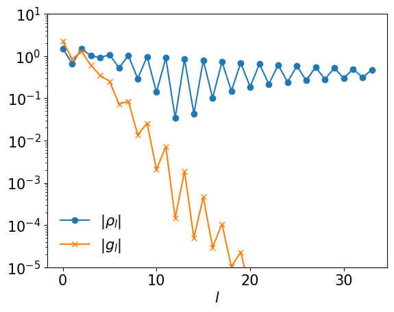
We consider a Green’s function genereated by poles:

\[ G(\mathrm{i}\nu) = \sum_{p=1}^{N_\mathrm{P}} \frac{c_p}{\mathrm{i}\nu - \omega_p}, \]

where \(\nu\) is a fermionic or bosonic Matsubara frequency. The corresponding specral function \(A(\omega)\) is given by

\[ A(\omega) = \sum_{p=1}^{N_\mathrm{P}} c_p \delta(\omega - \omega_p). \]

The modified (regularized) spectral function reads

\[\begin{split} \rho(\omega) = \begin{cases} \sum_{p=1}^{N_\mathrm{P}} c_p \delta(\omega - \omega_p) & \mathrm{(fermion)},\\ \sum_{p=1}^{N_\mathrm{P}} (c_p/\tanh(\beta \omega_p/2)) \delta(\omega - \omega_p) & \mathrm{(boson)}. \end{cases} \end{split}\]

for the logistic kernel. We immediately obtain

\[\begin{split} \rho_l = \begin{cases} \sum_{p=1}^{N_\mathrm{P}} c_p V_l(\omega_p) & \mathrm{(fermion)},\\ \sum_{p=1}^{N_\mathrm{P}} c_p V_l(\omega_p)/\tanh(\beta \omega_p/2))& \mathrm{(boson)}. \end{cases} \end{split}\]

The following code demostrates this transformation for bosons.

import sparse_ir
import numpy as np
%matplotlib inline
import matplotlib.pyplot as plt
plt.rcParams['font.size'] = 15

beta = 15
wmax = 10
basis_b = sparse_ir.FiniteTempBasis("B", beta, wmax, eps=1e-10)

coeff = np.array([1])
omega_p = np.array([0.1])

rhol_pole = np.einsum('lp,p->l', basis_b.v(omega_p), coeff/np.tanh(0.5*beta*omega_p))
gl_pole = - basis_b.s * rhol_pole

plt.semilogy(np.abs(rhol_pole), marker="o", label=r"$|\rho_l|$")
plt.semilogy(np.abs(gl_pole), marker="x", label=r"$|g_l|$")

plt.xlabel(r"$l$")
plt.ylim([1e-5, 1e+1])
plt.legend(frameon=False)
plt.show()

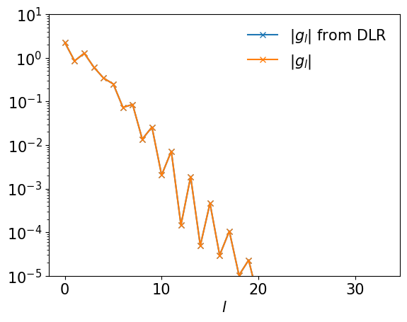
Alternatively, we can use DiscreteLehmannRepresentation

from sparse_ir.dlr import DiscreteLehmannRepresentation
dlr = DiscreteLehmannRepresentation(basis_b, omega_p)
gl_pole2 = dlr.to_IR(coeff/np.tanh(0.5*beta*omega_p))

plt.semilogy(np.abs(gl_pole2), marker="x", label=r"$|g_l|$ from DLR")
plt.semilogy(np.abs(gl_pole), marker="x", label=r"$|g_l|$")


plt.xlabel(r"$l$")
plt.ylim([1e-5, 1e+1])
plt.legend(frameon=False)
plt.show()

From smooth spectral function

For a smooth spectral function \(\rho(\omega)\), the expansion coefficients can be evaluated by computing the integral

\[ \rho_l = \int_{-\omega_\mathrm{max}}^{\omega_\mathrm{max}} \mathrm{d} \omega V_l(\omega) \rho(\omega). \]

One might consider to use the Gauss-Legendre quadrature. As seen in previous sections, the distribution of \(V_l(\omega)\) is much denser than Legendre polynomial \(P_l(x(\tau))\) around \(\tau=0, \beta\). Thus, evaluating the integral precisely requires the use of composite Gauss–Legendre quadrature, where the whole inteval \([-\omega_\mathrm{max}, \omega_\mathrm{max}]\) is divided to subintervals and the normal Gauss-Legendre quadrature is applied to each interval. The roots of \(V_l(\omega)\) for the highest \(l\) used in the expansion is a reasonable choice of the division points. If \(\rho(\omega)\) is smooth enough within each subinterval, the result converges exponentially with increasing the degree of the Gauss-Legendre quadrature.

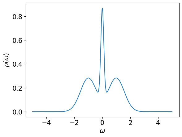
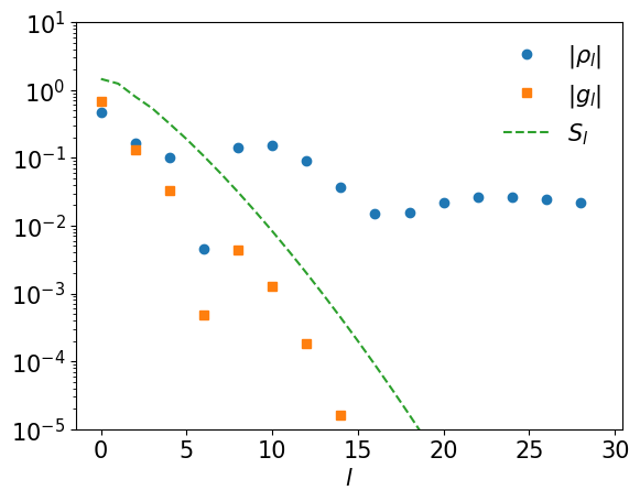
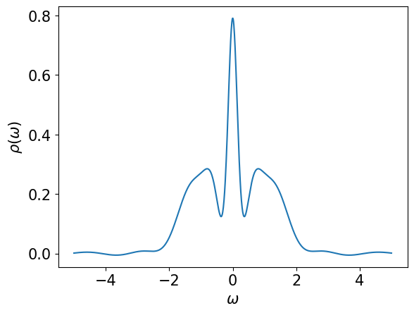
Below, we demonstrate how to compute \(\rho_l\) for a spectral function consisting of of three Gausssian peaks using the composite Gauss-Legendre quadrature. Then, \(\rho_l\) can be transformed to \(g_l\) by multiplying it with \(- S_l\).

# Three Gaussian peaks (normalized to 1)
gaussian = lambda x, mu, sigma:\
    np.exp(-((x-mu)/sigma)**2)/(np.sqrt(np.pi)*sigma)

rho = lambda omega: 0.2*gaussian(omega, 0.0, 0.15) + \
    0.4*gaussian(omega, 1.0, 0.8) + 0.4*gaussian(omega, -1.0, 0.8)

omegas = np.linspace(-5, 5, 1000)
plt.xlabel(r"$\omega$")
plt.ylabel(r"$\rho(\omega)$")
plt.plot(omegas, rho(omegas))
plt.show()

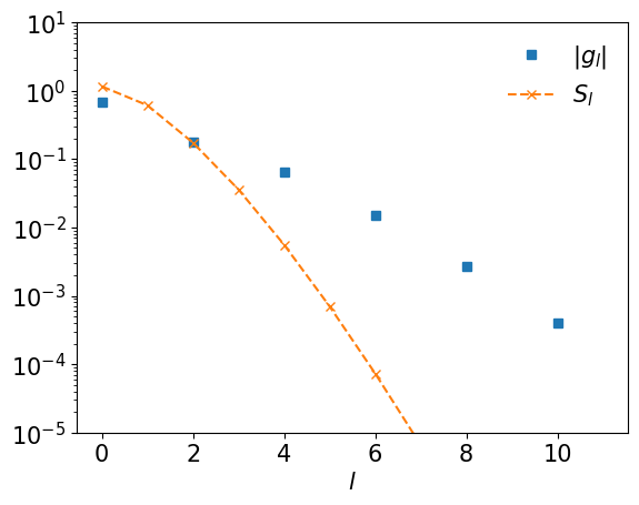
beta = 10
wmax = 10
basis = sparse_ir.FiniteTempBasis("F", beta, wmax, eps=1e-10)

rhol = basis.v.overlap(rho)
gl = - basis.s * rhol

plt.semilogy(np.abs(rhol), marker="o", ls="", label=r"$|\rho_l|$")
plt.semilogy(np.abs(gl), marker="s", ls="", label=r"$|g_l|$")
plt.semilogy(np.abs(basis.s), marker="", ls="--", label=r"$S_l$")
plt.xlabel(r"$l$")
plt.ylim([1e-5, 10])
plt.legend(frameon=False)
plt.show()
#plt.savefig("coeff.pdf")

\(\rho_l\) is evaluated on arbitrary real frequencies as follows.

rho_omgea_reconst = basis.v(omegas).T @ rhol

plt.xlabel(r"$\omega$")
plt.ylabel(r"$\rho(\omega)$")
plt.plot(omegas, rho_omgea_reconst)
plt.show()

From IR to imaginary time

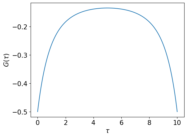
We are now ready to evaluate \(g_l\) on arbitrary \(\tau\) points. A naive way is as follows.

taus = np.linspace(0, beta, 1000)
gtau1 = basis.u(taus).T @ gl
plt.plot(taus, gtau1)
plt.xlabel(r"$\tau$")
plt.ylabel(r"$G(\tau)$")
plt.show()

Alternatively, we can use TauSampling as follows.

smpl = sparse_ir.TauSampling(basis, taus)
gtau2 = smpl.evaluate(gl)
plt.plot(taus, gtau1)
plt.xlabel(r"$\tau$")
plt.ylabel(r"$G(\tau)$")
plt.show()

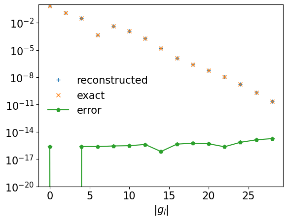
From full imaginary-time data

A numerically stable way to expand \(G(\tau)\) in IR is evaluating the integral

\[ G_l = \int_0^\beta \mathrm{d} \tau G(\tau) U_l(\tau). \]

You can use overlap function as well.

def eval_gtau(taus):
    uval = basis.u(taus) #(nl, ntau)
    if isinstance(taus, np.ndarray):
       print(uval.shape, gl.shape)
       return uval.T @ gl
    else:
       return uval.T @ gl

gl_reconst = basis.u.overlap(eval_gtau)

ls = np.arange(basis.size)
plt.semilogy(ls[::2], np.abs(gl_reconst)[::2], label="reconstructed", marker="+", ls="")
plt.semilogy(ls[::2], np.abs(gl)[::2], label="exact", marker="x", ls="")
plt.semilogy(ls[::2], np.abs(gl_reconst - gl)[::2], label="error", marker="p")
plt.xlabel(r"$l$")
plt.xlabel(r"$|g_l|$")
plt.ylim([1e-20, 1])
plt.legend(frameon=False)
plt.show()

Remark: What happens if \(\omega_\mathrm{max}\) is too small?

If \(G_l\) do not decay like \(S_l\), \(\omega_\mathrm{max}\) may be too small. Below, we numerically demonstrate it.

from scipy.integrate import quad

beta = 10
wmax = 0.5
basis_bad = sparse_ir.FiniteTempBasis("F", beta, wmax, eps=1e-10)

# We expand G(τ).
gl_bad = [quad(lambda x: eval_gtau(x) * basis_bad.u[l](x), 0, beta)[0] for l in range(basis_bad.size)]

plt.semilogy(np.abs(gl_bad), marker="s", ls="", label=r"$|g_l|$")
plt.semilogy(np.abs(basis_bad.s), marker="x", ls="--", label=r"$S_l$")
plt.xlabel(r"$l$")
plt.ylim([1e-5, 10])
#plt.xlim([0, basis.size])
plt.legend(frameon=False)
plt.show()
#plt.savefig("coeff_bad.pdf")

Matrix-valued object

evaluate and fit accept a matrix-valued object as an input. The axis to which the transformation applied can be specified by using the keyword augment axis.

np.random.seed(100)
shape = (1,2,3)
gl_tensor = np.random.randn(*shape)[..., np.newaxis] * gl[np.newaxis, :]
print("gl: ", gl.shape)
print("gl_tensor: ", gl_tensor.shape)

gl:  (30,)
gl_tensor:  (1, 2, 3, 30)

smpl_matsu = sparse_ir.MatsubaraSampling(basis)
gtau_tensor = smpl_matsu.evaluate(gl_tensor, axis=3)
print("gtau_tensor: ", gtau_tensor.shape)
gl_tensor_reconst = smpl_matsu.fit(gtau_tensor, axis=3)
assert np.allclose(gl_tensor, gl_tensor_reconst)

gtau_tensor:  (1, 2, 3, 30)