Orbital magnetic susceptibility#
Author: [Soshun Ozaki], [Takashi Koretsune]
Theory of the orbital magnetism#
The orbital magnetism is the magnetism induced by a vector potential coupled with the electron momentum, and is one of the fundamental thermodynamic properties of electron systems. A lot of efforts were dedicated to the formulation of the orbital magnetic susceptibility, and the simple but complete formula was derived by Fukuyama [1]. Recently, a new formula for the tight-binding model, which is based on the Peierls phase, has been derived and is applied to various lattice models[2,3,4]. The new formula is different from the Fukuyama formula [1] derived for the Bloch states in the continuum model. The relationship between them was clarified in [5] and [6]. In the continuum model, there are several contributions of the magnetic field to the orbital magnetic susceptibility in addition to the contribution from the Peierls phase. As far as the Peierls phase is concerned, the new formula will be correct.
Ref: [1] H. Fukuyama, Prog. Theor. Phys. 45, 704 (1971). [2] G. Gómez-Santos and T. Stauber, Phys. Rev. Lett. 106, 045504 (2011). [3] A. Raoux, F. Piéchon, J. N. Fuchs, and G. Montambaux, Phys. Rev. B 91, 085120 (2015). [4] F. Piéchon, A. Raoux, J.-N. Fuchs, and G. Montambaux, Phys. Rev. B 94, 134423 (2016). [5] M. Ogata and H. Fukuyama, J. Phys. Soc. Jpn. 84 124708 (2015). [6] H. Matsuura and M. Ogata, J. Phys. Soc. Jpn. 85 074709 (2016).
The orbital magnetic susceptibility formula#
The newly developed orbital magnetic susceptibility formula for tight-binding models is given by
where \(G=G(i\omega_n, {\boldsymbol k})\) is the thermal Green’s function for the tight-binding model, \(\gamma_i({\boldsymbol k})=\frac{\partial H_{\boldsymbol k}}{\partial k_i}, (i=x,y)\) and \(\gamma_{xy}({\boldsymbol k})= \frac{\partial^2 H_{\boldsymbol k}}{\partial k_x \partial k_y}\) represent the derivative of the tight-binding Hamiltonian \(H_{\boldsymbol k}\), and \(n\) summation represents the Matsubara summation. Since this formula is written in terms of the thermal Green’s functions, it is suitable for the demonstration of the Matsubara summation using the IR basis. We present codes for the computation of the orbital magnetic susceptibility using this formula for the tight-binding models on the two basic lattices, the square and honeycomb lattices with transfer integral \(t\), lattice constant \(a\). Note that the orbital magnetic susceptibility in the square (honeycomb) lattice is obtained in the tight-binding model [3] ([2]) and in the continuum model [7] ([8]), respectively. In our practical implementation, we perform the Matsubara summation using the ‘sparse ir’ package, and \({\boldsymbol k}\) summation over the Brillouin zone is evaluated by a simple discrete summation. We show the results as functions of the chemical potential.
Ref: [7] M. Ogata, J. Phys. Soc. of Jpn. 85, 064709 (2016). [8] M. Ogata, J. Phys. Soc. of Jpn. 85, 104708 (2016).
Code implementation#
We load basic modules used in the following.
!pip install sparse_ir
import numpy as np
import scipy
import itertools
import matplotlib.pyplot as plt
import sparse_ir
Requirement already satisfied: sparse_ir in /home/jovyan/.venv/default/lib/python3.11/site-packages (1.0.0)
Requirement already satisfied: numpy in /home/jovyan/.venv/default/lib/python3.11/site-packages (from sparse_ir) (1.25.0)
Requirement already satisfied: scipy in /home/jovyan/.venv/default/lib/python3.11/site-packages (from sparse_ir) (1.11.0)
Requirement already satisfied: setuptools in /home/jovyan/.venv/default/lib/python3.11/site-packages (from sparse_ir) (66.1.1)
Parameter setting#
We use the units of \(k_B=1\) in the following. We set \(t=a=1\) and \(T = 0.1\).
t = 1         # hopping amplitude
a = 1         # lattice constant
T = 0.1       # temperature
beta = 1/T
wmax = 10
nk1 = 200
nk2 = 200
IR_tol = 1e-10
mu_range = np.linspace(-4.5, 4.5, 91)
Function for the orbital magnetic susceptibility#
Here, we implement a function to calculate the orbital magnetic susceptibility from \(H_{\boldsymbol k}\), \(\gamma_x(\boldsymbol k)\), \(\gamma_y(\boldsymbol k)\), and \(\gamma_{xy}(\boldsymbol k)\). First, we calculate \(\chi(i \omega_n)\) for sampling Matsubara points and then obtain \(k_B T\sum_n \chi(i \omega_n)\) using the IR basis.
def orbital_chi(IR_basis_set, hkgk, klist, mu_range):
    smpl_iwn = IR_basis_set.smpl_wn_f.wn
    chi_iw = np.zeros((len(mu_range), len(smpl_iwn)), dtype=complex)
    for k in klist:
        hk, gx, gy, gxy = hkgk(k)
        ek, v = np.linalg.eigh(hk)
        vd = np.conj(v.T)
        giw = 1/(1j * np.pi/IR_basis_set.beta * smpl_iwn[None,None,:] - (ek[:,None,None] - mu_range[None,:,None]))
        gx = vd @ gx @ v
        gy = vd @ gy @ v
        gxy = vd @ gxy @ v
        chi_iw += np.einsum("ab, bmn, bc, cmn, cd, dmn, da, amn->mn",
                            gx, giw, gy, giw, gx, giw, gy, giw, optimize=True)
        chi_iw += (1/2) * np.einsum("ab, bmn, bc, cmn, ca, amn->mn",
                                    gx, giw, gy, giw, gxy, giw, optimize=True)
        chi_iw += (1/2) * np.einsum("ab, bmn, bc, cmn, ca, amn->mn",
                                    gy, giw, gx, giw, gxy, giw, optimize=True)
    chil = IR_basis_set.smpl_wn_f.fit(chi_iw, axis=1)
    smpl_tau0 = sparse_ir.TauSampling(IR_basis_set.basis_f, sampling_points=[0.0])
    chi_tau = smpl_tau0.evaluate(chil, axis=1)
    return chi_tau.real / len(klist)
We also implement a single band version of the function.
def orbital_chi1(IR_basis_set, hkgk, klist, mu_range):
    smpl_iwn = IR_basis_set.smpl_wn_f.wn
    chi_iw = np.zeros((len(mu_range), len(smpl_iwn)), dtype=complex)
    for k in klist:
        hk, gx, gy, gxy = hkgk(k)
        giw = 1/(1j * np.pi/IR_basis_set.beta * smpl_iwn[None,:] - (hk - mu_range[:,None]))
        chi_iw += gx**2 * gy**2 * giw**4
        chi_iw += gx * gy * gxy * giw**3
    chil = IR_basis_set.smpl_wn_f.fit(chi_iw, axis=1)
    smpl_tau0 = sparse_ir.TauSampling(IR_basis_set.basis_f, sampling_points=[0.0])
    chi_tau = smpl_tau0.evaluate(chil, axis=1)
    return chi_tau.real / len(klist)
We set the IR basis set and \(\boldsymbol k\) mesh.
IR_basis_set = sparse_ir.FiniteTempBasisSet(beta=beta, wmax=wmax, eps=IR_tol)
kx_list = np.arange(nk1)/nk1
ky_list = np.arange(nk2)/nk2
klist = np.array(list(itertools.product(kx_list, ky_list)))
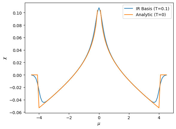
Two-dimensional square lattice#
Now, we evaluate the orbital magnetic susceptibility as a function of chemical potential, \(\chi(\mu)\), for the two-dimensional square lattice.
def hkgk_square(k):
    hk = -2 * t * (np.cos(2*np.pi*k[0]) + np.cos(2*np.pi*k[1]))
    gx = 2 * t * a * np.sin(2*np.pi*k[0])
    gy = 2 * t * a * np.sin(2*np.pi*k[1])
    gxy = 0
    return hk, gx, gy, gxy

chi_mu = orbital_chi1(IR_basis_set, hkgk_square, klist, mu_range)
For comparison, we calculate the analytic result at \(T=0\) [3,5].
k = 1 - mu_range**2/16
chi_anltc = np.where(k >= 0, -(scipy.special.ellipe(k)-scipy.special.ellipk(k)/2)*(2/3)/np.pi**2, 0)

plt.plot(mu_range, chi_mu, label='IR Basis (T=0.1)')
plt.plot(mu_range, chi_anltc, label='Analytic (T=0)')
plt.xlabel("$\mu$")
plt.ylabel("$\chi$")
plt.legend()
plt.show()
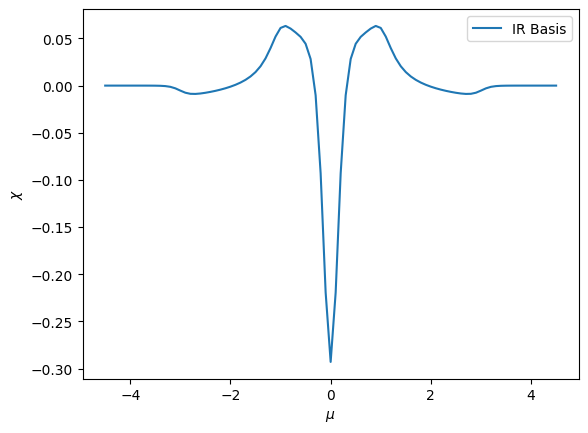
Graphene#
Next, we evaluate the orbital magnetic suscepitbility for graphene.
sq3 = np.sqrt(3)
def hkgk_graphene(k):
    kx, ky = 2*np.pi*k[0]/a, 2*np.pi*(k[0] + 2*k[1])/(a*sq3)
    h = -t * (np.exp(1j*ky*a/sq3) + 2 * np.cos(kx*a/2) * np.exp(-1j*ky*a/(2*sq3)))
    hk = np.array([ [ 0, h ], [ np.conj(h), 0 ] ])

    hx =  t * a * np.sin(kx/2) * np.exp(-1j*ky/(2*sq3))
    hy = -t * a * (1j/sq3 * (np.exp(1j*ky/sq3) - np.cos(kx/2) * np.exp(-1j*ky/(2*sq3))))
    gx = np.array([ [ 0, hx ], [ np.conj(hx), 0 ] ])
    gy = np.array([ [ 0, hy ], [ np.conj(hy), 0 ] ])

    hxy = -t * a * a * 1j/(2*sq3) * np.sin(kx/2) * np.exp(-1j*ky/(2*sq3))
    gxy = np.array([ [ 0, hxy ], [ np.conj(hxy), 0 ] ])

    return hk, gx, gy, gxy

chi_mu = orbital_chi(IR_basis_set, hkgk_graphene, klist, mu_range)
plt.plot(mu_range, chi_mu, label='IR Basis')
plt.xlabel("$\mu$")
plt.ylabel("$\chi$")
plt.legend()
plt.show()