Intermediate representation (IR)

\[ \newcommand{\iv}{{\mathrm{i}\nu}} \newcommand{\wmax}{{\omega_\mathrm{max}}} \newcommand{\dd}{{\mathrm{d}}} \]

One-particle Green’s function

We introduce a Green’s function with imaginary arguments in time and frequency. This has no physical meaning but a mere mathematical trick to make calculations easier (to give another example of this: in Minkowski spacetime we take advantage of a similiar substitution).

The so-called imaginary-frequency (Matsubara) Green’s functions are defined as follows:

\[ G_{ij}(\tau-\tau') = -\langle T_\tau [c_i(\tau){c}^\dagger_j(\tau')]\rangle, \]

where \(i\) and \(j\) denote spin/orbital/band and \(T_\tau\) is the time-ordering operator. Here, \(\tau\) represents a imaginary time unit \(\mathrm{i}t\), while \(c_i\)/\(c_j\) is a fermionic or bosonic annihilation/creation operator.

The Fourier Transformation of \(G_{ij}(\tau)\) (with \(\tau \in [0,\beta]\)) reads

\[ G_{ij}(\iv_n) = \int_0^{\beta} \dd \tau e^{\iv_n\tau} G_{ij}(\tau), \]

where \(\nu_n = (2n+1)\pi/\beta\) (fermion) and \(\nu_n = 2n\pi/\beta\) (boson) with \(n\) being an integer. The inverse temperature is denoted by \(\beta\) (We take \(\hbar=1\)). The inverse transformation is given by

\[ G_{ij}(\tau) = \frac{1}{\beta}\sum_{n=-\infty}^\infty e^{-\iv_n\tau}G_{ij}(\iv_n). \]

Continuing \(G_{ij}(\iv_n)\) to a holomorphic function in the upper half of the complex plane, the imaginary-frequency (Matsubara) Green’s function can be related to the “ordinary” retarded Green’s function as

\[ G_{ij}^\mathrm{R}(\omega)=G_{ij}(z \rightarrow \omega+\mathrm{i}0^{+}). \]

In the following, we omit the symbols \(i\), \(j\), \(n\) unless there is confusion.

Lehmann representation

In the imaginary-frequency domain, the Lehmann representation reads

\[ \begin{align} G(\iv) &= \int_{-\infty}^\infty \dd\omega \underbrace{\frac{1}{\iv - \omega}}_{\equiv K(\iv, \omega)} A(\omega), \end{align} \]

where \(A(\omega)\) is a spectral function. \(K(\iv, \omega)\) is the so-called analytic continuation kernel. The Lehmann representation can be transformed to the imaginary-time domain as

(1)\[ \begin{align} G(\tau) &= - \int_{-\infty}^\infty \dd\omega K(\tau, \omega) A(\omega), \end{align} \]

where \(0 < \tau < \beta\) and

\[\begin{split} \begin{align} K(\tau, \omega) &\equiv - \frac{1}{\beta} \sum_{\iv} e^{-\iv \tau} K(\iv, \omega) = \begin{cases} \frac{e^{-\tau\omega}}{1+e^{-\beta\omega}} & (\mathrm{fermion}),\\ \frac{e^{-\tau\omega}}{1-e^{-\beta\omega}} & (\mathrm{boson}) \end{cases}. \end{align} \end{split}\]

The minus sign originates from our convention \(K(\tau, \omega) > 0\). To avoid the divergence of the bosonic kernel at \(\omega=0\), we reformulate Eq. (1) as

\[ \begin{equation} G(\tau)= - \int_{-\infty}^\infty\dd{\omega} K^\mathrm{L}(\tau,\omega) \rho(\omega), \end{equation} \]

where \(K^\mathrm{L}(\tau, \omega)\) is the “logistic kernel” defined as

(2)\[ K^\mathrm{L}(\tau, \omega) = \frac{e^{-\tau\omega}}{1+e^{-\beta\omega}}, \]

and \(\rho(\omega)\) is the modified spectral function

\[\begin{split} \begin{align} \rho(\omega) &\equiv \begin{cases} A(\omega) & (\mathrm{fermion}),\\ \frac{A(\omega)}{\tanh(\beta \omega/2)} & (\mathrm{boson}). \end{cases} \end{align} \end{split}\]

Singular value expansion and basis functions

The singular value expnasion of the kernel (2) reads [Shinaoka et al., 2017]

\[ K^\mathrm{L}(\tau, \omega) = \sum_{l=0}^\infty U_l(\tau) S_l V_l(\omega), \]

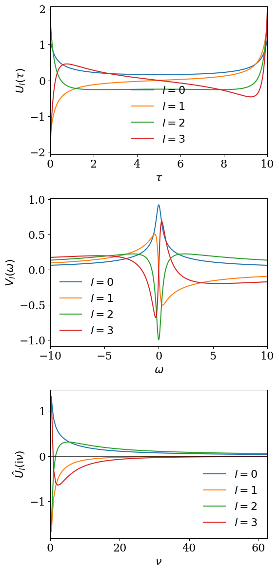
for \(\omega \in [-\wmax, \wmax]\) with \(\wmax\) (>0) being a cut-off frequency. \(U_l(\tau)\) and \(V_l(\omega)\) are left and right singular functions and \(S_l\) is the singular values (with \(S_0>S_1>S_2>...>0\)). The two sets of singular functions \(U\) and \(V\) make up the basis functions of the so-called Intermediate Representation (IR), which depends on \(\beta\) and the cutoff \(\wmax\). For the peculiar choice of the regularization for the bosonic kernel using \(K^\mathrm{L}\), these basis functions do not depend on statistical properties. The basis functions \(U_l(\tau)\) are transformed to the imaginary-frequency axis as

\[ U_l(\iv) \equiv \int_0^\beta \dd \tau e^{\iv \tau} U_l(\tau). \]

Some of the information regarding real-frequency properties of the system is often lost during transition into the imaginary-time domain, so that the imaginary-frequency Green’s function does hold less information than the real-frequency Green’s function. The reason for using IR lies within its compactness and ability to display that information in imaginary quantities.

The decay of the singular values depends on \(\beta\) and \(\wmax\) only through the dimensionless parameter \(\Lambda\equiv \beta\wmax\). The following plots show the singular values and the basis functions computed for \(\beta=10\) and \(\wmax=10\).

import numpy as np
%matplotlib inline
import matplotlib.pyplot as plt
import sparse_ir

plt.rcParams.update({
    "font.family": "serif",
    "font.size": 16,
})

lambda_ = 100
beta = 10
wmax = lambda_/beta
basis = sparse_ir.FiniteTempBasis('F', beta, wmax, eps=1e-10)

plt.semilogy(basis.s, marker='o', ls='')
plt.xlabel(r'$l$')
plt.ylabel(r'$S_l$')
plt.tight_layout()
plt.show()

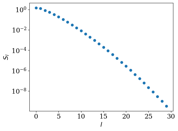
fig = plt.figure(figsize=(6,12))
ax1 = plt.subplot(311)
ax2 = plt.subplot(312)
ax3 = plt.subplot(313)
axes = [ax1, ax2, ax3]

taus = np.linspace(0, beta, 1000)
omegas = np.linspace(-wmax, wmax, 1000)

beta = 10
nmax = 100

v = 2*np.arange(nmax)+1
iv = 1J * (2*np.arange(nmax)+1) * np.pi/beta

uhat_val = basis.uhat(v)
for l in range(4):
    ax1.plot(taus, basis.u[l](taus), label=f'$l={l}$')
    ax2.plot(omegas, basis.v[l](omegas), label=f'$l={l}$')
    y = uhat_val[l,:].imag if l%2 == 0 else uhat_val[l,:].real
    ax3.plot(iv.imag, y, label=f'$l={l}$')

ax1.set_xlabel(r'$\tau$')
ax2.set_xlabel(r'$\omega$')
ax1.set_ylabel(r'$U_l(\tau)$')
ax2.set_ylabel(r'$V_l(\omega)$')
ax1.set_xlim([0,beta])
ax2.set_xlim([-wmax, wmax])

ax3.plot(iv.imag, np.zeros_like(iv.imag), ls='-', lw=0.5, color='k')
ax3.set_xlabel(r'$\nu$')
ax3.set_ylabel(r'$\hat{U}_l(\mathrm{i}\nu)$')
ax3.set_xlim([0, iv.imag.max()])

for ax in axes:
    ax.legend(loc='best', frameon=False)

plt.tight_layout()

We expand \(G(\tau)\) and \(\rho(\omega)\) as

\[ G(\tau) = \sum_{l=0}^{L-1} G_l U_l(\tau) + \epsilon_L, \]

\[ \hat{G}(\mathrm{i}\nu) = \sum_{l=0}^{L-1} G_l \hat{U}_l(\mathrm{i}\nu) + \hat{\epsilon}_L, \]

where \(\epsilon_L,~\hat{\epsilon}_L \approx S_L\). The expansion coefficients \(G_l\) can be determined from the spectral function as

\[ G_l = -S_l \rho_l, \]

where

\[ \rho_l = \int_{-\omega_\mathrm{max}}^{\omega_\mathrm{max}} \mathrm{d} \omega \rho(\omega) V_l(\omega). \]

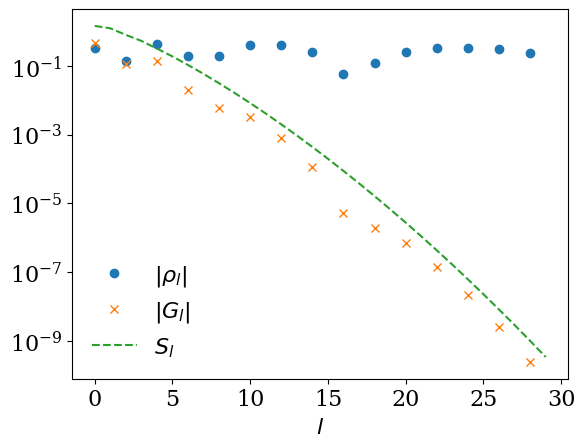
As a simple example, we consider a particle-hole-symmetric simple spectral function \(\rho(\omega) = \frac{1}{2} (\delta(\omega-1) + \delta(\omega+1))\) for fermions. The expansion coefficients are given by

\[ \rho_l = \frac{1}{2}(V_l(1) + V_l(-1)). \]

rho_l = 0.5 * (basis.v(1) + basis.v(-1))
gl = - basis.s * rho_l

ls = np.arange(basis.size)
plt.semilogy(ls[::2], np.abs(rho_l[::2]), label=r"$|\rho_l|$", marker="o", ls="")
plt.semilogy(ls[::2], np.abs(gl[::2]), label=r"$|G_l|$", marker="x", ls="")
plt.semilogy(ls, basis.s, label=r"$S_l$", marker="", ls="--")
plt.xlabel(r"$l$")
plt.legend(frameon=False)
plt.show()
#plt.savefig("plot.pdf")

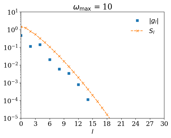
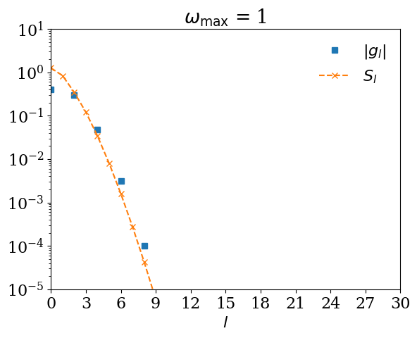
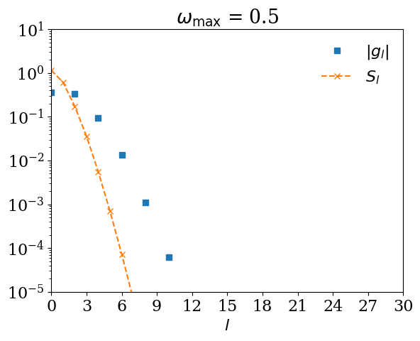
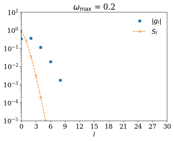
Remark: What happens if \(\omega_\mathrm{max}\) is too small?

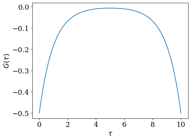
If you expand \(G(\tau)\) using \(U_l(\tau)\) for too small \(\omega_\mathrm{max}\), \(|G_l|\) decays slower than \(S_l\). Let us demonstrate it with \(\omega_\mathrm{max} = 0.5\).

def gtau_exact(tau):
    return -0.5*(np.exp(-tau)/(1 + np.exp(-beta)) + np.exp(tau)/(1 + np.exp(beta)))

plt.plot(taus, gtau_exact(taus))
plt.xlabel(r"$\tau$")
plt.ylabel(r"$G(\tau)$")
plt.show()
#plt.savefig("gtau.pdf")

from scipy.integrate import quad
from matplotlib.ticker import MaxNLocator

for wmax_bad in [10, 1, 0.5, 0.2]:
    basis_bad = sparse_ir.FiniteTempBasis("F", beta, wmax_bad, eps=1e-10)

    # We expand G(τ).
    gl_bad = [quad(lambda x: gtau_exact(x) * basis_bad.u[l](x), 0, beta)[0] for l in range(basis_bad.size)]

    ax = plt.figure().gca()
    ax.xaxis.set_major_locator(MaxNLocator(integer=True)) # Force xtics to be integer
    plt.semilogy(np.abs(gl_bad), marker="s", ls="", label=r"$|g_l|$")
    plt.semilogy(np.abs(basis_bad.s), marker="x", ls="--", label=r"$S_l$")
    plt.title(r"$\omega_\mathrm{max}$ = " + str(wmax_bad))
    plt.xlabel(r"$l$")
    plt.xlim([0, 30])
    plt.ylim([1e-5, 10])
    plt.legend(frameon=False)
    plt.show()
    #plt.savefig(f"coeff_bad_{wmax_bad}.pdf")