DMFT with IPT solver#
Author: Niklas Witt
In this tutorial, we will implement the Dynamical Mean-Field Theory (DMFT) using the iterative perturbation theory (IPT) as a solver for the impurity problem [1]. It is assumed that the reader is somewhat familiar with the concept of DMFT and the Anderson impurity model. Good resources to learn about this topic can be found, e.g., in Refs. [2-4].
Theory#
Model#
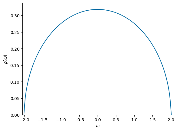
We compute a paramagnetic solution assuming the non-interacting semi-circular density of state (Bethe lattice)
at half filling. We set the hopping \(t_\star=1\), so that the half bandwitdh is \(D=2t_\star = 2\). Our goal is to find the Mott transition in this model. The non-interacting, local Green function is given by the spectral representation
with fermionic Matsubara frequencies \(\omega_n=(2n+1)\pi T\). We can directly compute this equation with the IR basis.
DMFT equations#
In DMFT, the self-energy is approximated by the local solution of an impurity model. The self-consistent equations to be solved are the Dyson equation of the interacting local Green function \(G_{\mathrm{loc}}\)
with the self-energy \(\Sigma\) (from the impurity problem) and the cavity Green function/Weiss field \(\mathcal{G}\) as well as the mean-field mapping for the Bethe lattice [2]
for which the impurity problem needs to be solved. As a starting point we put in \(G^0_{\mathrm{loc}}(i\omega_n)\) into the latter equation.
IPT Solver#
The IPT is an inexpensive way of solving the impurity problem (instead of applying e.g. Quantum Monte Carlo (QMC) or Exact Diagonalization (ED) methods). The self-energy is approximated by the second-order perturbation theory (SOPT/GF2, see other tutorial)
with the Hubbard interaction \(U\) and imaginary time \(\tau\). Note that we absorbed the constant Hartree term \(\Sigma_H = U n_{\sigma} = U\frac{n}{2}\) into the definition of the chemical potential \(\mu\) (at half filling, it is shifted to zero). Otherwise we would have to treat this term separately, since the IR basis cannot model the \(\delta\)-peak in frequency space well/compactly. In this case, evaluate the term analytically and add it after the Fourier transformation step.
Renormalization factor#
The Mott transition can be detected by monitoring the renormalization factor
In the non-interacting limit \(U\rightarrow 0\) we have \(Z\rightarrow 1\). Correlation effects reduce \(Z\) as \(Z < 1\) and the Mott transition is signaled by a jump \(Z\to0\).
[1] A. Georges and G. Kotliar, Phys. Rev. B 45, 6479 (1992)
[2] A. Georges et al., Rev. Mod. Phys. 68, 13 (1996)
[3] Many book chapters of the Jülich autumn school series, see https://www.cond-mat.de/events/correl.html
[4] R. M. Martin, L. Reining, D. M. Ceperley, Interacting Electrons, Cambridge University Press (2016)
Notes on practical implementation#
We will try to find the Mott transition which is a phase transition of first order. To illustrate this, we will do calculations starting from the metallic and the insulating phase at the end of this tutorial. This will show a hysteresis, signaling the metastable/coexistence region of both solutions. For converged results, this will need many iteration steps.
In the insulating phase, the low-frequency part of the self-energy turns downwards and diverges. Using the above formula for calculating the renormalization factor \(Z\) from a linearized self-energy, it would be negative. To circumvent this unphysical notion, \(Z\) then is defined as zero in the implementation.
We include a mixing \(p<1\) in each iteration step, such that the Green function of step \(n+1\) is partially constructed from the old and new Green function as \(G^{n+1} = p\,G^{n+1} + (1-p)\,G^{n}\). This smoothes too strong oscillations of the solution which is important especially near the phase transition point.
Code implementation#
import numpy as np
import scipy as sc
import scipy.optimize
from warnings import warn
import sparse_ir
%matplotlib inline
import matplotlib.pyplot as plt
plt.style.use('tableau-colorblind10')
Setting up the solver#
Generating meshes#
We need to generate IR basis functions on a sparse \(\tau\) and \(i\omega_n\) grid. In addition, we set calculation routines to Fourier transform \(\tau\leftrightarrow i\omega_n\) (via IR basis).
# Initiate fermionic and bosonic IR basis objects by using (later):
# IR_basis_set = sparse_ir.FiniteTempBasisSet(beta, wmax, eps=IR_tol)
class Mesh:
    """
    Holding class for sparsely sampled imaginary time 'tau' / Matsubara frequency 'iwn' grids.
    Additionally it defines the Fourier transform via 'tau <-> l <-> wn'.
    """
    def __init__(self,IR_basis_set):
        self.IR_basis_set = IR_basis_set

        # lowest Matsubara frequency index
        self.iw0_f = np.where(self.IR_basis_set.wn_f == 1)[0][0]
        self.iw0_b = np.where(self.IR_basis_set.wn_b == 0)[0][0]

        # frequency mesh (for plotting Green function/self-energy)
        self.iwn_f = 1j * self.IR_basis_set.wn_f * np.pi * T

    def smpl_obj(self, statistics):
        """ Return sampling object for given statistic """
        smpl_tau = {'F': self.IR_basis_set.smpl_tau_f, 'B': self.IR_basis_set.smpl_tau_b}[statistics]
        smpl_wn  = {'F': self.IR_basis_set.smpl_wn_f,  'B': self.IR_basis_set.smpl_wn_b }[statistics]
        return smpl_tau, smpl_wn

    def tau_to_wn(self, statistics, obj_tau):
        """ Fourier transform from tau to iwn via IR basis """
        smpl_tau, smpl_wn = self.smpl_obj(statistics)

        obj_l   = smpl_tau.fit(obj_tau, axis=0)
        obj_wn  = smpl_wn.evaluate(obj_l, axis=0)
        return obj_wn

    def wn_to_tau(self, statistics, obj_wn):
        """ Fourier transform from iwn to tau via IR basis """
        smpl_tau, smpl_wn = self.smpl_obj(statistics)

        obj_l   = smpl_wn.fit(obj_wn, axis=0)
        obj_tau = smpl_tau.evaluate(obj_l, axis=0)
        return obj_tau
IPT solver#
We write a function for the IPT solver. We use the Mesh class defined above to perform calculation steps.
def IPTSolver(mesh, g_weiss, U):
    """
    IPT solver to calculate the impurity problem.
    Input:
        mesh - Holding class of IR basis with sparsely sampled grids.
        g_weiss - Weiss field of the bath (\mathcal(G); cavity Green function)
                  on Matsubara frequencies iwn.
        U - Hubbard interaction strength
    """

    # Fourier transform to imaginary time
    gtau = mesh.wn_to_tau('F', g_weiss)

    # Self-energy in SOPT
    sigma = U**2 * gtau**3

    # Fourier transform back to Matsubara frequency
    sigma = mesh.tau_to_wn('F', sigma)
    return sigma
DMFT loop#
We wrap the DMFT loop in a class that sets all necessary quantities when initializing and runs when calling the .solve instance.
class DMFT_loop:
    def __init__(self,mesh, g0_loc, U, D, sfc_tol=1e-4, maxiter=20, mix=0.2,
                  verbose=True):

        # Set input
        self.mesh = mesh
        self.U = U
        self.t = D/2
        self.mix = mix
        self.sfc_tol = sfc_tol
        self.maxiter = maxiter
        self.verbose = verbose

        # Initial Green function (e.g. non-interacting)
        self.g_loc = g0_loc

        # Initiate Weiss field
        self.sigma = 0
        self.calc_g_weiss()

    def solve(self):
        for it in range(self.maxiter):
            sigma_old = self.sigma

            # Solve impurity problem in IPT
            sigma = IPTSolver(self.mesh, self.g_weiss, self.U)
            self.sigma = sigma*mix + self.sigma*(1-mix)

            # Set new Green function and Weiss field
            self.calc_g_loc()
            self.calc_g_weiss()

            # Check whether solution is converged
            sfc_check = np.sum(abs(self.sigma-sigma_old))/np.sum(abs(self.sigma))
            if self.verbose:
                print(it, sfc_check)
            if sfc_check < self.sfc_tol:
                if self.verbose:
                    print("DMFT loop converged at desired accuracy of", self.sfc_tol)
                break

    def calc_g_loc(self):
        # Set interacting local Green function from Dyson's equation.
        self.g_loc = (self.g_weiss**(-1) - self.sigma)**(-1)

    def calc_g_weiss(self):
        # Calculate Weiss mean field of electron bath.
        self.g_weiss = (self.mesh.iwn_f - self.t**2 * self.g_loc)**(-1)
        #self.g_weiss = (self.g_loc**(-1) + self.sigma)**(-1)
Calculations#
Parameter setting#
### System parameters
D    = 2      # half bandwidth D = W/2 ; hopping t = 1 here
wmax = 2*D    # set wmax >= W = 2*D
T    = 0.1/D  # temperature
beta = 1/T    # inverse temperature
U    = 5.     # Hubbard interaction

### Numerical parameters
IR_tol  = 1e-15  # desired accuracy for l-cutoff of IR basis functions
maxiter = 300    # maximal number of DMFT convergence steps
sfc_tol = 1e-5   # desired accuracy of DMFT convergence
mix     = 0.25   # mixing factor
### Initialize calculation
# Set mesh
IR_basis_set = sparse_ir.FiniteTempBasisSet(beta, wmax, eps=IR_tol)
mesh = Mesh(IR_basis_set)

# Calculate non-interacting Green function
rho = lambda omega : 2*np.sqrt(D**2 - omega.clip(-D,D)**2)/(np.pi*D**2)
rho_l = IR_basis_set.basis_f.v.overlap(rho)
g0_l  = -IR_basis_set.basis_f.s * rho_l
g0_loc = IR_basis_set.smpl_wn_f.evaluate(g0_l)

# Initiate DMFT loop
solver = DMFT_loop(mesh, g0_loc, U, D, sfc_tol=sfc_tol, maxiter=maxiter, mix=mix, verbose=True)

# perform DMFT calculations
solver.solve()
0 1.0
1 0.4526747668336244
2 0.26493595064106534
3 0.17712860649742412
4 0.12506086096213812
5 0.09230256725264989
6 0.06979019823464438
7 0.053934867913427456
8 0.04227192248431622
9 0.03357001205305884
10 0.02691849039674672
11 0.021780606404512546
12 0.01775339770279033
13 0.01456954051980396
14 0.012027586033398159
15 0.009983392596860022
16 0.008327397213775567
17 0.006977578428932369
18 0.005870782942216203
19 0.004958407997128745
20 0.0042025099307517865
21 0.0035733390830017804
22 0.0030473652027623427
23 0.002605877222124777
24 0.0022338993660161515
25 0.0019193817067253973
26 0.0016525753516393664
27 0.0014255535425504499
28 0.0012318393774386576
29 0.0010661159416726041
30 0.0009239988579873411
31 0.0008018571118814759
32 0.0006966711221956847
33 0.0006059198206882623
34 0.0005274903829999142
35 0.00045960574982273025
36 0.0004007661730561527
37 0.0003497018696906231
38 0.0003053345083058815
39 0.00026674574865554493
40 0.0002331514361239665
41 0.00020388034850995704
42 0.00017835662235022703
43 0.00015608516530653385
44 0.00013663950154733107
45 0.00011965160738301257
46 0.00010480338139668624
47 9.181946214401839e-05
48 8.046116109789647e-05
49 7.05213220558007e-05
50 6.181995297107967e-05
51 5.420050408184711e-05
52 4.752668865441998e-05
53 4.167976078387961e-05
54 3.655617940062201e-05
55 3.206559959005401e-05
56 2.8129142096569938e-05
57 2.4677899894423794e-05
58 2.165164728798586e-05
59 1.899772245760746e-05
60 1.6670058871335322e-05
61 1.462834477425142e-05
62 1.283729315054671e-05
63 1.1266007326510936e-05
64 9.887429927721198e-06
DMFT loop converged at desired accuracy of 1e-05
Visualize results#
# Plot spectral function/density of states
omega = np.linspace(-D-0.01, D+0.01,200)
plt.plot(omega, rho(omega),'-')
ax = plt.gca()
ax.set_xlim([-D-0.05,D+0.05])
ax.set_ylim([0,2/np.pi/D+0.02])
ax.set_xlabel('$\\omega$')
ax.set_ylabel('$\\rho(\\omega)$')
plt.show()
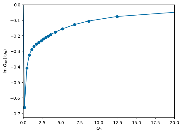
# plot frequency dependence of Green function
plt.plot(np.imag(mesh.iwn_f), np.imag(solver.g_loc),'-o')
ax = plt.gca()
ax.set_xlabel('$\\omega_n$')
ax.set_xlim([0,20])
ax.set_ylabel('Im $G_{\\mathrm{loc}}(i\\omega_n)$')
ax.set_ylim(ymax=0)
plt.show()
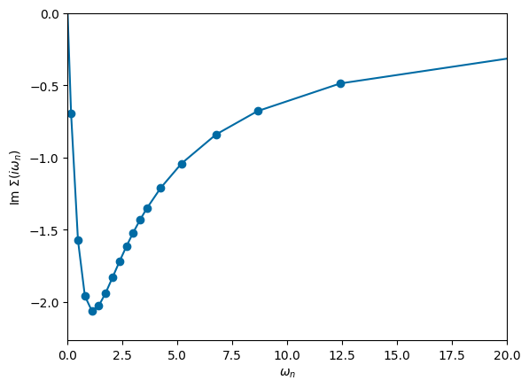
# plot frequency dependence of self-energy
plt.plot(np.imag(mesh.iwn_f), np.imag(solver.sigma),'-o')
ax = plt.gca()
ax.set_xlabel('$\\omega_n$')
ax.set_xlim([0,20])
ax.set_ylabel('Im $\\Sigma(i\\omega_n)$')
ax.set_ylim(ymax=0)
plt.show()
Renormalization factor#
We calculate the renormalization factor from a linearized self-energy. It is also possible to approximate it from the lowest Matsubara frequency (see and try out the difference!).
def CalcRenormalizationZ(solver):
    sigma = solver.sigma
    sigma_iw0 = sigma[solver.mesh.iw0_f]
    sigma_iw1 = sigma[solver.mesh.iw0_f+1]
    beta = solver.mesh.IR_basis_set.beta
    Z = 1/(1 - np.imag(sigma_iw1 - sigma_iw0)*beta/(2*np.pi))
    #Z = 1/(1 - np.imag(sigma_iw0)*beta/np.pi)

    # When system turns insulating, slope becomes positive/Z becomes negative -> set Z to zero then
    if Z < 0:
        Z = 0
    return Z
Now we perform calculations for different \(U\) to find the Mott transition. To see the evolution, we also plot the self-energy for some \(U\) values.
# Set U values as unit of t
U_min = 0
U_max = 6.5
U_num = 66
U_arr = np.linspace(U_min, U_max, U_num)
Z_arr = np.empty(U_arr.shape)

# Set new convergence parameters to achieve good convergence near the phase transition line
maxiter = 1500    # maximal number of DMFT convergence steps
sfc_tol = 1e-14   # desired accuracy of DMFT convergence


# Set mesh
IR_basis_set = sparse_ir.FiniteTempBasisSet(beta, wmax, eps=IR_tol)
mesh = Mesh(IR_basis_set)

# Calculate noninteracting Green function
rho = lambda omega : np.sqrt(D**2 - omega.clip(-D,D)**2)/(np.pi*D)
rho_l = IR_basis_set.basis_f.v.overlap(rho)
g0_l  = -IR_basis_set.basis_f.s * rho_l
g0_loc = IR_basis_set.smpl_wn_f.evaluate(g0_l)


plt.figure()
for it, U in enumerate(U_arr):
    # Starting from non-interacting solution
    solver = DMFT_loop(mesh, g0_loc, U, D, sfc_tol=sfc_tol, maxiter=maxiter, mix=mix, verbose=False)
    solver.solve()
    Z = CalcRenormalizationZ(solver)
    Z_arr[it] = Z

    if it in [30, 34, 35, 36, 37, 40]:
        plt.plot(np.imag(mesh.iwn_f[mesh.iw0_f:]), np.imag(solver.sigma[mesh.iw0_f:]),'-o', label='$U$={:.2f}'.format(U))


ax = plt.gca()
ax.set_xlabel('$\\omega_n$')
ax.set_xlim([0,4])
ax.set_ylabel('Im $\\Sigma(i\\omega_n)$')
ax.set_ylim(ymax=0)
ax.legend()

#%%%%%%%%%%%%%%%% Plot results
plt.figure()
plt.plot(U_arr, Z_arr, '--o')
ax = plt.gca()
ax.set_xlabel('$U/t_\\star$', fontsize=12)
ax.set_xlim([U_min, U_max])
ax.set_ylabel('$Z = (1-\partial\Sigma/\partial\omega)^{-1}$', fontsize=12)
ax.set_ylim([0,1])
plt.show()
/tmp/ipykernel_5389/4134521955.py:34: RuntimeWarning: invalid value encountered in scalar divide
  sfc_check = np.sum(abs(self.sigma-sigma_old))/np.sum(abs(self.sigma))
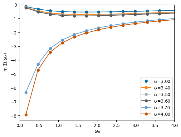
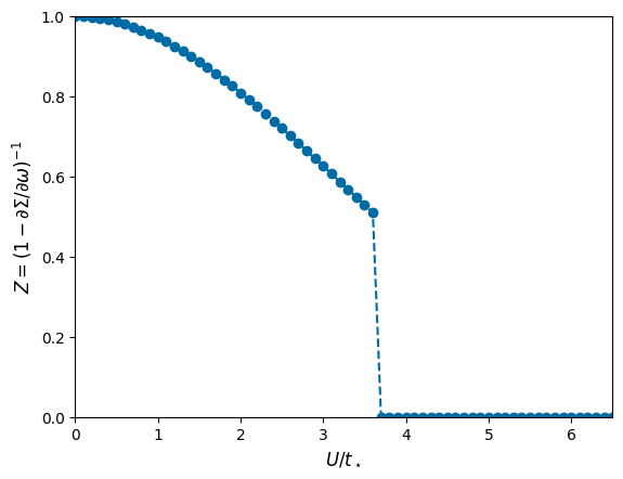
You can quite well see a jump of \(Z\) between \(U/t_\star=3\) and 4 which is accompanied by the low-frequency part of the self-energy diverging instead of going to zero.
In a last step, we want to map out the metastable coexistence region. In order to do this, we have to start every new \(U\) calculation from the previous converged solution. If we start from small \(U\), we start from the metallic region, whereas starting from large \(U\) corresponds to starting from the insulating solution.
Z_arr_mt = np.empty(U_arr.shape)
Z_arr_in = np.empty(U_arr.shape)

for it in range(len(U_arr)):
    if it != 0:
        solver_mt = DMFT_loop(mesh, solver_mt.g_loc, U_arr[it], D, sfc_tol=sfc_tol, maxiter=maxiter, mix=mix, verbose=False)
        solver_in = DMFT_loop(mesh, solver_in.g_loc, U_arr[U_num-1-it], D, sfc_tol=sfc_tol, maxiter=maxiter, mix=mix, verbose=False)
    else:
        solver_mt = DMFT_loop(mesh, g0_loc, U_arr[it], D, sfc_tol=sfc_tol, maxiter=maxiter, mix=mix, verbose=False)
        solver_in = DMFT_loop(mesh, g0_loc, U_arr[U_num-1-it], D, sfc_tol=sfc_tol, maxiter=maxiter, mix=mix, verbose=False)

    solver_mt.solve()
    Z = CalcRenormalizationZ(solver_mt)
    Z_arr_mt[it] = Z

    solver_in.solve()
    Z = CalcRenormalizationZ(solver_in)
    Z_arr_in[U_num-1-it] = Z


#%%%%%%%%%%%%%%%% Plot results
plt.figure()
plt.plot([],[],'w',label='Starting pt.')
plt.plot(U_arr, Z_arr, '--o', label='$G_0$')
plt.plot(U_arr, Z_arr_in, '--x', label='$G_{\\mathrm{insulating}}$')
plt.plot(U_arr, Z_arr_mt, '--^', label='$G_{\\mathrm{metal}}$')
ax = plt.gca()
ax.set_xlabel('$U/t_\\star$', fontsize=12)
ax.set_xlim([U_min, U_max])
ax.set_ylabel('$Z = (1-\partial\Sigma/\partial\omega)^{-1}$', fontsize=12)
ax.set_ylim([0,1])
ax.legend(fontsize=12)
plt.show()
/tmp/ipykernel_5389/4134521955.py:34: RuntimeWarning: invalid value encountered in scalar divide
  sfc_check = np.sum(abs(self.sigma-sigma_old))/np.sum(abs(self.sigma))
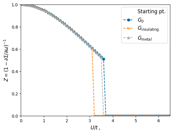
For comparison, we also plotted the transition line where we always start from the non-interacting Green function \(G_0\). Since we do only a few iteration steps, we do not have completetly converged solutions, so that the \(G_0\) line has a slightly larger critical \(U\) value compared to the line which starts from the metallic solution. Try increasinging the parameter maxiter (to 1000 or so) and decreasing the parameter sfc_tol (to 1e-14 or so) and look at the results! (The lines should become equal.)
Often the energy unit is not the hopping \(t_\star\) but the half-bandwidth \(D\), so we can also plot the results in this convention:
#%%%%%%%%%%%%%%%% Plot results
plt.figure()
plt.plot([],[],'w',label='Starting pt.')
plt.plot(U_arr/D, Z_arr, '--o', label='$G_0$')
plt.plot(U_arr/D, Z_arr_in, '--x', label='$G_{\\mathrm{insulating}}$')
plt.plot(U_arr/D, Z_arr_mt, '--^', label='$G_{\\mathrm{metal}}$')
ax = plt.gca()
ax.set_xlabel('$U/D$', fontsize=12)
ax.set_xlim([U_min/D, U_max/D])
ax.set_ylabel('$Z = (1-\partial\Sigma/\partial\omega)^{-1}$', fontsize=12)
ax.set_ylim([0,1])
ax.legend(fontsize=12)
plt.show()
