Estimation of exchange interactions

Estimation of exchange interactions#

Liechtenstein method#

The Liechtenstein method is a method for deriving the classical spin models from the itinerant electron models. Initially developed by Liechtenstein et al.[1] in the framework of the spin density functional theory, the method has been applied to various systems and is successful in understanding many magnetic behaviors, including finite temperature effects and long-period magnetic structures, which are not accessible from the spin density functional theory alone. Here, as the simplest case, we will see the formulation for the single-orbital model, where we can use the sparse_ir library to accelerate the calculations.

Liechtenstein formula in single-orbital model#

Let us consider to derive exchange interactions from the following one-body Hamiltonian:

\begin{array}{r} H = - t \sum_{< i, j >} \sum_{s} c_{i s}^{†} c_{j s} - \sum_{i} \sum_{s s^{'}} c_{i s}^{†} (B_{i} \cdot σ_{s s^{'}}) c_{i s^{'}} \end{array}

If we set the effective magnetic field $B_{i}$ to $B_{i} = J S e_{i} / 2$ , this is a classical Kondo lattice model, while if $B_{i} = U m_{i} / 2$ , this is a Hubbard model with the mean-field approximation. The basic idea of the Liechtenstein method is to impose the equivalence of the spin-angle-derivatives of the total energies in the itinerant systems and the classical spin systems. Note that the derivatives generally depend on a reference magnetic structure. Here, let us consider the classical Heisenberg model $E = - 2 \sum_{< i, j >} J_{i j} e_{i} \cdot e_{j}$ as a spin model and the $\hat{z}$ -polarized ferromagnetic state (namely, $B_{i} = B \hat{z}$ ) as a reference magnetic structure. Then, we will get

\begin{array}{r} J_{i j} = - B^{2} T \sum_{ω_{n}} G_{i j, +} (i ω_{n}) G_{j i, -} (i ω_{n}) \end{array}

where the Green function $G_{i j, σ} (i ω_{n})$ is a Fourier transform of $G_{k, σ} (i ω_{n}) = [i ω_{n} - (ε_{k} - B σ - μ)]^{- 1}$ with the single-particle dispersion $ε_{k}$ and chemical potential $μ$ . $i ω_{n} = (2 n + 1) π T$ is the Matsubara frequency and $k$ is the crystal momentum. An important quantity here is defined by $J_{0} = \sum_{0 \neq i} J_{0 i}$ , which is related to the mean-filed transition temperature $T_{c}^{m f}$ in the classical Heisenberg model by $T_{c}^{m f} = 2 J_{0} / 3$ . This can be evaluated from the above $J_{i j}$ , or the direct comparison of the second derivatives of the total energy, which gives

\begin{array}{r} J_{0} = \frac{B}{2} (n_{0, +} - n_{0, -}) + B^{2} T \sum_{ω_{n}} G_{00, +} (i ω_{n}) G_{00, -} (i ω_{n}) \end{array}

In practice, $G_{00, σ} (i ω_{n})$ can be obtained by the $k$ summation of $G_{k, σ} (i ω_{n})$ since all sites are equivalent in this model. Thus, the number of operations is $O (N_{M} N_{k}^{t o t})$ where $N_{M}$ is the number of Matsubara frequency and $N_{k}^{t o t}$ is the total number of k-points. Since the typical value of $N_{M}$ is $N_{M} \sim β W$ , the total cost is given by $O (β W N_{k})$ . On the other hand, we need $G_{i j, +} (i ω_{n})$ to evaluate $J_{i j}$ , and in this case, the number of operations becomes $O (N_{M} (N_{k} \ln N_{k})^{d})$ since the Fourier transform requires $N_{k} \ln N_{k}$ operations for a single axis, where $N_{k}$ is the number of k-points for a single axis and $d$ is the dimension. Thus, we need $O (β W (N_{k} \ln N_{k})^{d})$ in total.

Sparse_ir#

Since $G_{i j, σ} (i ω_{n})$ as well as $G_{00, σ} (i ω_{n})$ are just linear conbinations of $G_{k, σ} (i ω_{n})$ , all terms we need take the following form,

\begin{array}{r} \frac{1}{i ω_{n} - ε_{a}} \frac{1}{i ω_{n} - ε_{b}} = \frac{1}{ε_{a} - ε_{b}} (\frac{1}{i ω_{n} - ε_{a}} - \frac{1}{i ω_{n} - ε_{b}}) \end{array}

Thus, we can expand $G_{i j, +} (i ω_{n}) G_{j i, -} (i ω_{n})$ in the expression for $J_{i j}$ and $G_{00, +} (i ω_{n}) G_{00, -} (i ω_{n})$ for $J_{0}$ by the intermadiate representation. Since the summation over $i ω_{n}$ is equivalent to evaluating the Fourier transform at $τ = 0$ , we need only $O (\ln (β W))$ operations for the Matsubara frequancy axis. Thus, the computational cost becomes $O (\ln (β W) N_{k}^{t o t})$ for $J_{0}$ and $O (\ln (β W) (N_{k} \ln N_{k})^{d})$ for $J_{i j}$ .

Code implementation#

Here, let us see an example code in a square lattice tight-binding model with dispersion $ε_{k} = - 2 t [\cos (k_{x}) + \cos (k_{y})]$ . First, we load all necessary modules that we need:

import numpy as np
%matplotlib inline
import matplotlib.pyplot as plt
import matplotlib.cm as cm
import sparse_ir

Parameter setting#

The parameters to define the system are as follows; $t$ : the nearest-neighbor hopping amplitude, $β$ : the inverse temperature, $N_{k}$ : the numer of k-poitns for a single-axis and $B$ : the strengh of the effective magnetic field.

t = 1 # means the bandwidth W is W=8t in a square lattice model
beta = 50 # inverse temperature
nk = 36 # number of k-points for a signle-axis
b_eff = 3 # strength of the effective magnetic field

Liechtenstein solver#

This class contains two solvers, j0_calc for calculation of $J_{0}$ and jij_calc for $J_{i j}$ . Both can be called after instantiating the class.

class liechtenstein:
  def __init__(self, basis, *args):
    # constructor of liechtenstein class
    # the class requires five arguments: sparse_ir basis object, t, beta, nk, and b_eff
    
    self.basis, self.M, self.T = basis, sparse_ir.MatsubaraSampling(basis), sparse_ir.TauSampling(basis)
    t, self.beta, self.nk, self.b_eff= args[0], args[1], args[2], args[3]
    k1, k2 = np.meshgrid(np.arange(self.nk)/self.nk, np.arange(self.nk)/self.nk, indexing='ij')
    self.ek = -2* t * (np.cos(2*np.pi*k1) + np.cos(2*np.pi*k2))
    self.nkt = self.nk**2

  def j0_calc(self, e_range=np.zeros(1), NM=None):
    # solver to evaluate J_0
    # e_range: numpy ndarray object to specify the chemical potentials at which we evaluate J_0
    # NM: maximum number of Matsubara frequency. if None, sparse sampling will be used
  
    # set Matsubara frequency grid
    if NM is None: iw = 1j*np.pi*self.M.sampling_points/self.beta
    else         : iw = 1j*np.pi*(2*np.arange(-NM,NM)+1)/self.beta

    # calculate the first term in the expresson of J_0
    n_up = .5 * (1-np.tanh(.5*self.beta*(self.ek[None,:,:]-e_range[:,None,None]-self.b_eff)))
    n_dn = .5 * (1-np.tanh(.5*self.beta*(self.ek[None,:,:]-e_range[:,None,None]+self.b_eff)))
    j0_1 = .5 * self.b_eff * np.mean(n_up - n_dn, axis=(1,2))
        
    # calculate the second term in the expression of J_0 as a function of iw 
    gkio_up = 1/(iw[:,None,None,None] - (self.ek[None,None,:,:]-self.b_eff-e_range[None,:,None,None]))
    gkio_dn = 1/(iw[:,None,None,None] - (self.ek[None,None,:,:]+self.b_eff-e_range[None,:,None,None]))
    gio_up = np.mean(gkio_up, axis=(2,3))
    gio_dn = np.mean(gkio_dn, axis=(2,3))
    j0_2_w = self.b_eff**2 * gio_up * gio_dn
    
    # evaluate a summation over iw 
    if NM is None:
      j0_2_l = self.M.fit(j0_2_w.reshape(len(iw),len(e_range))) # transform to the intermediate representation
      j0_2 = self.basis.u(0)@j0_2_l # evaluate the function at \tau=0
    else:
      j0_2 = np.sum(j0_2_w,axis=0)/self.beta
    
    # sum up the two terms
    self.j0 = np.real(j0_1 + j0_2)
    self.j0_e_range = e_range

  def jij_calc(self, mu=0, NM=None):
    # solver to evaluate J_ij
    # mu: the chemical potential at which we evaluate J_ij
    # NM: maximum number of Matsubara frequency. if None, sparse sampling will be used
    
    # set Matsubara frequency grid
    if NM is None: iw = 1j*np.pi*self.M.sampling_points/self.beta
    else         : iw = 1j*np.pi*(2*np.arange(-NM,NM)+1)/self.beta
        
    # calculate J_ij as a function of iw 
    gkio_up = 1/(iw[:,None,None] - (self.ek[None,:,:]-self.b_eff-mu))
    gkio_dn = 1/(iw[:,None,None] - (self.ek[None,:,:]+self.b_eff-mu))
    grio_up = np.fft.fftn(gkio_up,axes=(1,2))/self.nkt
    grio_dn = np.fft.ifftn(gkio_dn,axes=(1,2))
    jij_w = - self.b_eff**2 * grio_up * grio_dn
    
    # evaluate a summation of J_ij over iw 
    if NM is None:
      jij_l = self.M.fit(jij_w.reshape(len(iw),self.nkt))
      jij = self.basis.u(0)@jij_l
    else:
      jij = np.sum(jij_w,axis=0)/self.beta
    
    # arrange the format to ouput the data
    self.jij = np.real(jij)
    self.jij[0] = 0
    self.jij_r = np.linalg.norm(np.array(np.meshgrid(np.arange(self.nk),np.arange(self.nk), indexing='ij')), axis=0).flatten()

Instantiation#

In the instantation, we have to pass a sparse_ir.basis object as the first argument of the liechtenstein class.

Lambda = 2*max(8*t, b_eff) * beta
basis = sparse_ir.FiniteTempBasis(statistics='F', beta=beta, wmax=Lambda, eps=1e-7)
l = liechtenstein(basis, t, beta, nk, b_eff)

Executing the solver for J_0#

Here, let us evaluate J_0 as a function of the chemmical potential $μ$ . To check the validity of the sparse sampleing method, we will compare it with that evaluated by the conventional Matsubara frequency grid. This can be done as follows:

plt.xlabel("mu")
plt.ylabel("J_0")
for i, nm in enumerate([100, 200, 400, 800, 1600]):
      l.j0_calc(e_range=np.linspace(-10,10,41), NM=nm)
      plt.plot(l.j0_e_range, l.j0, marker='.', label=str(nm), color=cm.cool(i/5.))
l.j0_calc(e_range=np.linspace(-10,10,41))
plt.plot(l.j0_e_range, l.j0, marker='.', label='Sparse_IR', color=cm.cool(1.0))
plt.legend()
plt.show()

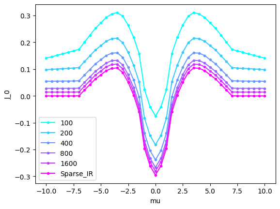
../_images/a1aaae0521f14dbbb0ae86e601ebf9756f4ac3f0bd2ab937a79c9347701c3b08.png

As is expected, the system favors the antiferromagnetic state at the half-filling while it favors the ferromagnetic state at the low-carrier regime. This feature is consistent with the super-exchange and the doule-exchange interactions.

Executing the solver for J_ij#

We can also evaluate J_ij by using jij_calc function as follows.

plt.clf
plt.xlabel("distance")
plt.ylabel("J_ij")
plt.xlim([0,5])
l.jij_calc(0)
plt.scatter(l.jij_r, l.jij, marker='.')
plt.show()

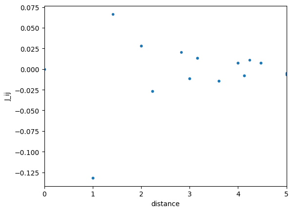
../_images/e9d354a234a2915910edfea46a6262e639f886b7cb4cbb8b9d50cef28168b7a2.png

We can easily check $J_{0} = \sum_{j} J_{0 j}$ as follows.

J0_1 = l.j0[20]   # J0 at mu=0 evaluated by j0_calc
J0_2 = sum(l.jij)  
print(J0_1,J0_2)

-0.2954591400058828 -0.2954591398013725

[1] Liechtenstein et al., J. Phys. F: Met. Phys. 14 L125 (1984).