SpM analytic continuation

Author: Kazuyoshi Yoshimi & Junya Otsuki

This example provides an application of sparse-ir to the sparse-modeling analytic continuation (SpM) algorithm. We reproduce the result presented in the original paper [Otsuki et al., 2017].

The analytic continuation can be formulated as the inverse problem of the equation

(3)\[ G(\tau) = -\int_{-\infty}^{\infty} d\omega K(\tau, \omega) \rho(\omega). \]

We evaluate \(\rho(\omega)\) for a given \(G(\tau)\).

Preparation

!pip install sparse_ir
!pip install admmsolver

We use a sample data provided in the repository SpM-lab/SpM.

# Download data for G(tau) and rhow(omega) from GitHub repo
from urllib.request import urlretrieve
base_url = "https://raw.githubusercontent.com/SpM-lab/SpM/master/samples/fermion/"
for name in ["Gtau.in", "Gtau.in.dos"]:
    urlretrieve(base_url + name, name)
# Alternatively, we can use the following command:
#!wget https://raw.githubusercontent.com/SpM-lab/SpM/master/samples/fermion/Gtau.in
#!wget https://raw.githubusercontent.com/SpM-lab/SpM/master/samples/fermion/Gtau.in.dos

import numpy as np
%matplotlib inline
import matplotlib.pyplot as plt

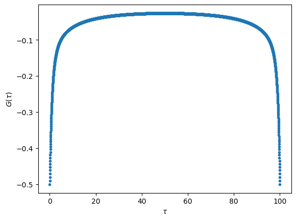
Input data for \(G(\tau)\)

We load the sample data provided in the repository SpM-lab/SpM.

#Load Gtau
Gtau = np.loadtxt("Gtau.in")[:, 2]

# Set imaginary-time
beta = 100
ntau = len(Gtau)
ts = np.linspace(0.0, beta, ntau)

Let us plot the input data loaded.

# Plot G(tau)
fig, ax = plt.subplots()
ax.plot(ts, Gtau, '.')
ax.set_xlabel(r"$\tau$")
ax.set_ylabel(r"$G(\tau)$")
plt.show()

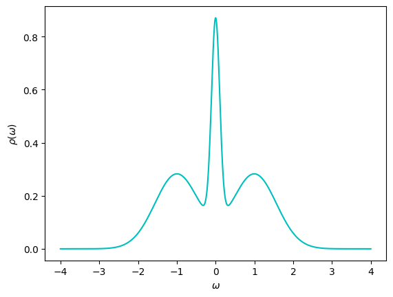
Spectral function \(\rho(\omega)\) (answer)

We generate the real frequency grid for the spectral function \(\rho(\omega)\)

#Set omega
Nomega = 1001
omegamin = -4
omegamax = 4
ws = np.linspace(-omegamax, omegamax, num=Nomega)

The exact spectrum is provided as well. The spectrum is plotted below.

rho_answer = np.loadtxt("Gtau.in.dos")[:, 1]

# Plot rho(omega)
fig, ax = plt.subplots()
ax.plot(ws, rho_answer, '-c')
ax.set_xlabel(r"$\omega$")
ax.set_ylabel(r"$\rho(\omega)$")
plt.show()

IR basis

We first generate IR basis. On a discrete grid of \(\{ \tau_i \}\) and \(\{ \omega_j \}\), the kernel function \(K(\tau, \omega)\) are represented by a matrix \(\hat{K}\) with \(\hat{K}_{ij}=K(\tau_i, \omega_j)\). The singular value decomposition of \(\hat{K}\) defines the IR basis

\[ \hat{K} = \hat{U} \hat{S} \hat{V}^\mathrm{T}, \]

where

\[ \hat{U}_{il}=U_l(\tau_i), \quad \hat{S}_{ll} = S_l, \quad \hat{V}_{jl}=V_l(\omega_j). \]

The matrices \(\hat{U}\), \(\hat{S}\), and \(\hat{V}\) can be computed by sparse_ir.FiniteTempBasis class (https://sparse-ir.readthedocs.io/en/latest/basis.html).

import sparse_ir

#Set basis
SVmin = 1e-10
basis = sparse_ir.FiniteTempBasis(
            statistics="F", beta=beta, wmax=omegamax, eps=SVmin
        )
U = basis.u(ts).T
S = basis.s
V = basis.v(ws).T

U and V are two-dimensional ndarray (matrices), while S is a one-dimensional ndarray. Let us confirm it by printing the shapes explictly.

print(f"{U.shape}, {S.shape}, {V.shape}")

(4001, 43), (43,), (1001, 43)

SpM analytic continuation

The spectral function \(\rho(\omega)\) can be expanded with the IR basis

\[ \rho(\omega) = \sum_l \rho_l V_l(\omega) \]

The SpM analytic continuation algorithm evaluates the coefficient \(\{ \rho_l \}\). Eq. (3) is rewritten in terms of the IR basis by

\[ G(\tau_i) = \sum_l \hat{U}_{il} S_l \rho_l \]

We represent this equation with the conventional notation

\[ \boldsymbol{y} =A \boldsymbol{x}, \]

where

\[ y_i = -G(\tau_i), \quad A_{il}\equiv \hat{U}_{il} S_l, \quad x_l = \rho_l. \]

Here, \(\boldsymbol{y}\) is an input, and \(\boldsymbol{x}\) is the quantity to be evaluated.

y = -Gtau
A = np.einsum("il,l->il", U, S)

SpM evaluates \(\boldsymbol{x}\) by solving the optimization problem

\[ \boldsymbol{x}^{\ast} = \underset{\boldsymbol{x}}{\mathrm{arg\,min}} F(\boldsymbol{x}), \]

where

\[ F(\boldsymbol{x}) = \frac{1}{2} \| \boldsymbol{y} - A\boldsymbol{x} \|_2^2 + \lambda \| \boldsymbol{x} \|_1 + \infty \| C\boldsymbol{x} - D \|_2^2 + \infty \Theta (-V\boldsymbol{x}). \]

The first term is the least square fitting to the input, the second term is \(L_1\)-norm regularization, and the third term and the fourth term represent constraints: sum-rule and non-negativity, respectively.

An obtained solution depends on the value of the regularization parameter \(\lambda\), which should be optimized based on data science. But, for simplicity, we fix the value of \(\lambda\) in this example.

Note: In the original SpM paper, the least-square term is evaluated directly in the IR. Namely, using \(\hat{U}\hat{U}^{\dagger}=1\), the least-square term can be converted to

\[ \frac{1}{2} \| \boldsymbol{y} - A\boldsymbol{x} \|_2^2 = \frac{1}{2} \sum_l (G_l - S_l \rho_l)^2. \]

Because \(\hat{U}\) is not a unitary matrix in the present formalism, one cannot use this equation.

ADMM

We solve the above multi-constaint optimization problem using alternating direction method of multipliers (ADMM). To this end, we consider an alternative multivariate optimization problem

\[ \min_{\boldsymbol{x}_0, \boldsymbol{x}_1, \cdots} \tilde{F}(\boldsymbol{x}_0, \boldsymbol{x}_1, \cdots), \]

subject to equality conditions

\[ E_{ji} \boldsymbol{x}_i = E_{ij} \boldsymbol{x}_j. \]

Here, the objective function \(F\) is given by

\[ \tilde{F}(\boldsymbol{x}_0, \boldsymbol{x}_1, \cdots) = \sum_i F_i(\boldsymbol{x}_i) \]

We use admmsolver package. The import statement below shows all necessary classes for implementing the present optimization problem. Note that admmsolver is under active development and its interface is subject to future changes.

import admmsolver
import admmsolver.optimizer
import admmsolver.objectivefunc
from admmsolver.objectivefunc import (
    L1Regularizer,
    #LeastSquares,
    ConstrainedLeastSquares,
    NonNegativePenalty,
)
from admmsolver.matrix import identity
from admmsolver.optimizer import SimpleOptimizer
print(f"admmsolver=={admmsolver.__version__}")

admmsolver==0.7.6

\(L_2\) norms

The Green’s function follows the sum-rule

\[ \int_{-\infty}^{\infty} d\omega \rho(\omega) = 1 \]

More generally (including the self-energy), the right-hand side is given by \(-G(\tau=+0) - G(\tau=\beta-0)\), which is non-zero for orbital-diagonal components and 0 for off-diagonal components. In the IR basis, the left-hand side is reprenseted by

\[ \int_{-\infty}^{\infty} d\omega \rho(\omega) = G(\tau=-0) - G(\tau=0^+) = \sum_l [U_l(\tau=+0) + U_l(\tau=\beta-0) ] S_l \rho_l. \]

This sum-rule can be imposed by an infinite penalty. Together with the least-square term, we obtain

\[ F_0(\boldsymbol{x}_0) = \frac{1}{2} \| \boldsymbol{y} - A\boldsymbol{x}_0 \|_2^2 + \infty \| C\boldsymbol{x}_0 - D \|_2^2. \]

These \(L_2\) norm terms are implemented as admmsolver.objectivefunc.ConstrainedLeastSquares object.

# sum-rule
rho_sum = y[0] + y[-1]
C = (A[0] + A[-1]).reshape(1, -1)
lstsq_F = ConstrainedLeastSquares(0.5, A=A, y=y, C=C, D=np.array([rho_sum]))

\(L_1\)-norm regularization

The \(L_1\)-norm regularization term

\[ F_1(\boldsymbol{x}_1) = \lambda \| \boldsymbol{x}_1 \|_1 \]

is implemented as admmsolver.objectivefunc.L1Regularizer object. We note that \(\boldsymbol{x}_1\) will be finaly converged to \(\boldsymbol{x}_0\).

lambda_ = 10**-1.8  # regularization parameter
l1_F = L1Regularizer(lambda_, basis.size)

Here, we use \(\lambda=10^{-1.8}\), which was found to be optimal for the present dataset.

Non-negative constraint

The last term describes the non-negative constraint

\[ \rho(\omega) \geq 0 \]

Since we have the relation \(\rho(\omega_i)=(\hat{V}\boldsymbol{x})_i\), this inequality can be represented as a function

\[ F_2(\boldsymbol{x}_2) = \infty \Theta (-\boldsymbol{x}_2) \]

We note that \(\boldsymbol{x}_2 = V\boldsymbol{x}_0\) will be imposed later.

nonneg_F = NonNegativePenalty(Nomega)

We now define admmsolver.optimizer.Problem by integrating the three obejective functions.

objective_functions = [lstsq_F, l1_F, nonneg_F]
equality_conditions = [
    (0, 1, identity(basis.size), identity(basis.size)),
    # (0, 2, V.T, identity(Nomega)),
    (0, 2, V, identity(Nomega)),
]

p = admmsolver.optimizer.Problem(objective_functions, equality_conditions)

objective_functions is a list of functions \(F_0(\boldsymbol{x}_0)\), \(F_0(\boldsymbol{x}_1)\), \(F_0(\boldsymbol{x}_2)\). Two equality condition is set to equality_conditions. The first one denotes \(\boldsymbol{x}_0 = \boldsymbol{x}_1\), and the second one denotes \(V\boldsymbol{x}_0=\boldsymbol{x}_2\). Thus, the multivariate objective function \(\tilde{F}(\boldsymbol{x}_0, \boldsymbol{x}_1, \boldsymbol{x}_2)\) is reduced to the original objective function \(F(\boldsymbol{x})\).

We solve the problem defined above using admmsolver.optimizer.SimpleOptimizer.

maxiteration = 1000
initial_mu = 1.0
opt = SimpleOptimizer(p, mu=initial_mu)  # initialize solver
opt.solve(maxiteration)  # solve

Here, mu is a parameter which controls the convergence, and maxiteration is the maximum number of iterations.

The converged result is stored in opt.x, which is a list of vectors \(\boldsymbol{x}_0\), \(\boldsymbol{x}_1\), and \(\boldsymbol{x}_2\). We can access each vector by

x0, x1, x2 = opt.x
print(f"{x0.shape}, {x1.shape}, {x2.shape}")

(43,), (43,), (1001,)

The spectral function \(\rho(\omega)\) can be reconstructed from the coefficients \(\{ \rho_l \}\) stored in \(\boldsymbol{x}_0\).

rho = V @ x0

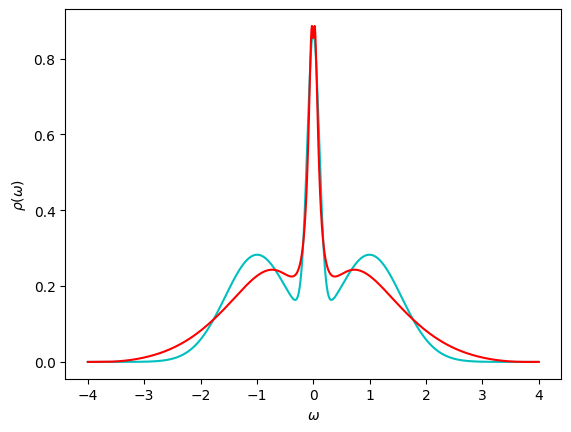
Plot the results

We plot the spectral function \(\rho(\omega)\) computed in the SpM together with the exact solution.

fig, ax = plt.subplots()
ax.plot(ws, rho_answer, '-c')
ax.plot(ws, rho.real, '-r')
ax.set_xlabel(r"$\omega$")
ax.set_ylabel(r"$\rho(\omega)$")
plt.show()

# save results
# specfile = "spectrum.dat"
# with open(specfile, "w") as f:
#     f.write(f"# log_lambda = f{lambdalog}\n")
#     for w, r in zip(ws, rho):
#         f.write(f"{w} {np.real(r)}\n")