Numerical analytic continuation

One of the main problems one faces when working with imaginary (Euclidean) time is inferring the real-time spectra \(\rho(\omega)\) from imaginary-time data \(G(\tau)\), in other words, we are seeking the inverse of the following Fredholm equation:

\[ G(\tau) = -\int d\omega\ K(\tau, \omega)\ \rho(\omega) = -\sum_{l=0}^\infty U_l(\tau)\ S_l \int d\omega\ V_l(\omega)\ \rho(\omega), \]

where again \(S_l\) are the singular values and \(U_l(\tau)\) and \(V_l(\omega)\) are the left and right singular (IR basis) functions, the result of a singular value expansion of the kernel \(K\).

Using the IR basis expansion, we can “invert” above equation to arrive at:

\[ \rho(\omega) \sim -\int d\tau\ K^{-1}(\omega, \tau)\ G(\tau) = -\sum_{l=0}^\infty V_l(\omega)\ \frac 1{S_l} \int d\tau\ U_l(\tau)\ G(\tau), \]

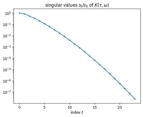
where \(K^{-1}\) denotes the pseudoinverse of \(K\). (We will defer questions about the exact nature of this inverse.) The numerical analytical continuation problem is now evident: The kernel is regular, i.e., all the singular values \(S_l > 0\), so the above equation can be evaluated analytically. However, \(S_l\) drop exponentially quickly, so any finite error, even simply the finite precision of \(G(\tau)\) in a computer, will be arbitrarily amplified once \(l\) becomes large enough. We say the numerical analytical continuation problem is ill-posed.

import numpy as np
import matplotlib.pyplot as pl
import sparse_ir

beta = 40.0
wmax = 2.0
basis = sparse_ir.FiniteTempBasis('F', beta, wmax, eps=2e-8)

pl.semilogy(basis.s / basis.s[0], '-+')
pl.title(r'singular values $s_\ell/s_0$ of $K(\tau, \omega)$')
pl.xlabel(r'index $\ell$');

Least squares form

In order to make meaningful progress, let us reformulate the analytic continutation as a least squares problem:

\[ \min_\rho \int d\tau\ \Big| G(\tau) + \int d\omega\ K(\tau, \omega)\ \rho(\omega) \Big|^2, \]

To simplify and speed up this equation, we want to use the IR basis form of the kernel. For this, remember that for any imaginary-time propagator:

\[ G(\tau) = \sum_{l=0}^{L-1} g_l U_l(\tau) + \epsilon_L(\tau), \]

where the error term \(\epsilon_L\) drops as \(S_L/S_0\). We can now choose the basis cutoff \(L\) large enough such that the error term is consistent with the intrinsic accuracy of the \(G(\tau)\), e.g., machine precision. (If there is a covariance matrix, generalized least squares should be used.) Since the IR basis functions \(U_l\) form an isometry, we also have that:

\[ \int\ d\tau\ |G(\tau)|^2 = \sum_{l=0}^{L-1} |g_l|^2 + O(\epsilon_L) \]

allowing us to truncate our analytic continuation problem to (cf. Jarrell and Gubernatis, 1996):

\[ \min_\rho \sum_{l=0}^{L-1} \Big| g_l + S_l \int d\omega\ V_l(\omega)\ \rho(\omega) \Big|^2. \qquad(1) \]

This already is an improvement over many analytical continuation algorithms, as it maximally compresses the observed imaginary-time data \(g_l\) without relying on any a priori discretizations of the kernel.

def semicirc_dos(w):
    return 2/np.pi * np.sqrt((np.abs(w) < wmax) * (1 - np.square(w/wmax)))

def insulator_dos(w):
    return semicirc_dos(8*w/wmax - 4) + semicirc_dos(8*w/wmax + 4)

# For testing, compute exact coefficients g_l for two models
rho1_l = basis.v.overlap(semicirc_dos)
rho2_l = basis.v.overlap(insulator_dos)
g1_l = -basis.s * rho1_l
g2_l = -basis.s * rho2_l

# Put some numerical noise on both of them (30% of basis accuracy)
rng = np.random.RandomState(4711)
noise = 0.3 * basis.s[-1] / basis.s[0]
g1_l_noisy = g1_l + rng.normal(0, noise, basis.size) * np.linalg.norm(g1_l)
g2_l_noisy = g2_l + rng.normal(0, noise, basis.size) * np.linalg.norm(g2_l)

Truncated-SVD regularization

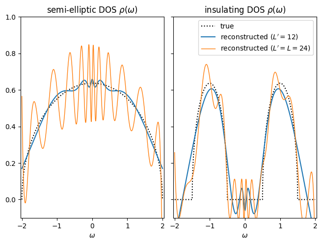
However, the problem is still ill-posed. As a first attempt to cure it, let us turn to truncated-SVD regularization (Hansen, 1987), by demanding that the spectral function \(\rho(\omega)\) is representable by the right singular functions:

\[ \rho(\omega) = \sum_{l=0}^{L'-1} \rho_l V_l(\omega), \]

where \(L' \le L\). The analytic continuation problem (1) then takes the following form:

\[ \rho_l = -g_l / S_l. \]

The choice of \(L'\) is now governed by a bias–variance tradeoff: as we increase \(L'\), more and more features of the spectral function emerge by virtue of \(\rho_l\), but at the same time \(1/S_l\) amplifies the stastical errors more strongly.

# Analytic continuation made (perhaps too) easy
rho1_l_noisy = g1_l_noisy / -basis.s
rho2_l_noisy = g2_l_noisy / -basis.s

w_plot = np.linspace(-wmax, wmax, 1001)
Vmat = basis.v(w_plot).T
Lprime1 = basis.size // 2

def _plot_one(subplot, dos, rho_l, name):
    pl.subplot(subplot)
    pl.plot(w_plot, dos(w_plot), ":k", label="true")
    pl.plot(w_plot, Vmat[:, :Lprime1] @ rho_l[:Lprime1],
            label=f"reconstructed ($L' = {Lprime1}$)")
    pl.plot(w_plot, Vmat @ rho_l, lw=1,
            label=f"reconstructed ($L' = L = {basis.size}$)")
    pl.xlabel(r"$\omega$")
    pl.title(name)
    pl.xlim(-1.02 * wmax, 1.02 * wmax)
    pl.ylim(-.1, 1)

_plot_one(121, semicirc_dos, rho1_l_noisy, r"semi-elliptic DOS $\rho(\omega)$")
_plot_one(122, insulator_dos, rho2_l_noisy, r"insulating DOS $\rho(\omega)$")
pl.legend()
pl.gca().set_yticklabels([])
pl.tight_layout(pad=.1, w_pad=.1, h_pad=.1)

Regularization

Above spectra are, in a sense, the best reconstructions we can achieve without including any more a priori information about \(\rho(\omega)\). However, it turns out we often know (or can guess at) quite a lot of properties of the spectrum:

1. the spectrum must be non-negative, \(\rho(\omega) \ge 0\), for one orbital, and positive semi-definite, \(\rho(\omega) \succeq 0\), in general,

2. the spectrum must be a density: \(\int d\omega\ \rho(\omega) = 1\),

3. one may assume that the spectrum may be “sensible”, i.e., not deviate too much from a default model \(\rho_0(\omega)\) (MAXENT) or not be too complex in structure (SpM/SOM).

These constraints are often encoded into the least squares problem (1) by restricting the space of valid solutions \(\mathcal R\) and by including a regularization term \(f_\mathrm{reg}[\rho]\):

\[ \min_{\rho\in\mathcal R}\bigg[ \sum_{l=0}^{L-1} \Big| g_l + S_l \int d\omega\ V_l(\omega)\ \rho(\omega) \Big|^2 + f_\mathrm{reg}[\rho] \bigg]. \qquad(2) \]

All of these constraints act as regularizers.

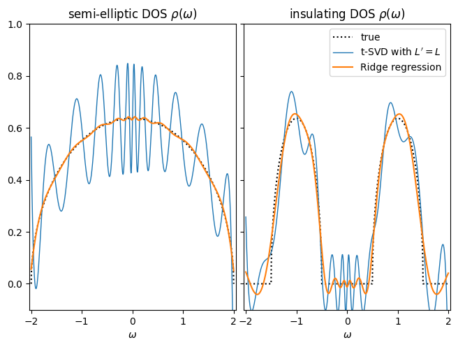
As a simple example, let us consider Ridge regression in the above problem. We again expand the spectral function in the right singular functions with \(L'=L\), but include a regularization term:

\[ f_\mathrm{reg}[\rho] = \alpha \sum_{l=0}^{L-1} | \rho_l |^2, \]

where \(\alpha\) is a hyperparameter (ideally tuned to the noise level). This term prevents \(\rho_l\) becoming too large due to noise amplification. The regularized least squares problem (2) then amounts to:

\[ \rho_l = -\frac{s_l}{s^2_l + \alpha^2} g_l \]

# Analytic continuation made (perhaps too) easy
alpha = 100 * noise
invsl_reg = -basis.s / (np.square(basis.s) + np.square(alpha))
rho1_l_reg = invsl_reg * g1_l_noisy
rho2_l_reg = invsl_reg * g2_l_noisy

def _plot_one(subplot, dos, rho_l, rho_l_reg, name):
    pl.subplot(subplot)
    pl.plot(w_plot, dos(w_plot), ":k", label="true")
    pl.plot(w_plot, Vmat @ rho_l, lw=1, label=f"t-SVD with $L'=L$")
    pl.plot(w_plot, Vmat @ rho_l_reg, label=f"Ridge regression")
    pl.xlabel(r"$\omega$")
    pl.title(name)
    pl.xlim(-1.02 * wmax, 1.02 * wmax)
    pl.ylim(-.1, 1)


_plot_one(121, semicirc_dos, rho1_l_noisy, rho1_l_reg, r"semi-elliptic DOS $\rho(\omega)$")
_plot_one(122, insulator_dos, rho2_l_noisy, rho2_l_reg, r"insulating DOS $\rho(\omega)$")
pl.legend()
pl.gca().set_yticklabels([])
pl.tight_layout(pad=.1, w_pad=.1, h_pad=.1)

Real-axis basis

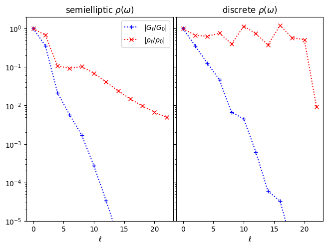
One problem we are facing when solving the regularized least squares problem (2) is that the regularization might “force” values of \(g_l\) well below the threshold \(L\). (For example, in general infinitely many \(g_l\) need to conspire to ensure that the spectral function is non-negative.) This is a problem because, unlike \(g_l\), which decay quickly by virtue of \(S_l\), the expansion coefficients \(\rho_l\) are not compact (see also Rothkopf, 2013):

Let us illustrate the decay of \(\rho_l\) for two densities of states:

1. semielliptic (left), where the \(\rho_l\) decay roughly as \(1/l\), and are thus not compact.

2. discrete set of peaks: \(\rho(\omega) \propto \sum_i \delta(\omega - \epsilon_i)\) (right), where \(\rho_l\) does not decay at all, signalling the fact that a delta-peak cannot be represented by any finite (or even infinite) expansion in the basis.

dos3 = np.array([-0.6, -0.1, 0.1, 0.6]) * wmax
rho3_l = basis.v(dos3).sum(1)
g3_l = -basis.s * rho3_l

def _plot_one(subplot, g_l, rho_l, title):
    pl.subplot(subplot)
    n = np.arange(0, g_l.size, 2)
    pl.semilogy(n, np.abs(g_l[::2]/g_l[0]), ':+b', label=r'$|G_\ell/G_0|$')
    pl.semilogy(n, np.abs(rho_l[::2]/rho_l[0]), ':xr', label=r'$|\rho_\ell/\rho_0|$')
    pl.title(title)
    pl.xlabel('$\ell$')
    pl.ylim(1e-5, 2)

_plot_one(121, g1_l, rho1_l, r'semielliptic $\rho(\omega)$')
pl.legend()
_plot_one(122, g3_l, rho3_l, r'discrete $\rho(\omega)$')
pl.gca().set_yticklabels([])
pl.tight_layout(pad=.1, w_pad=.1, h_pad=.1)

Thus, we need another representation for the real-frequency axis. The simplest one is to choose a grid \(\{\omega_1,\ldots,\omega_M\}\) of frequencies and a function \(f(x)\) and expand:

\[ \rho(\omega) = \sum_{m=1}^M a_i f(\omega - \omega_i), \]

where \(a_i\) are now the expansion coefficients. (More advanced methods also optimize over \(\omega_m\) and/or add some shape parameter of \(f\) to the optimization parameters.)

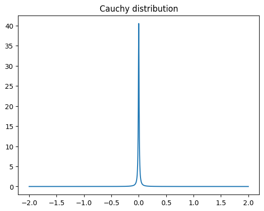
It is useful to use some probability distribution as \(f(x)\), as this allows one to translate non-negativity and norm of \(\rho(\omega)\) to non-negativity and norm of \(a_i\). Since one can only observe “broadened” spectra in experiment for any given temperature, a natural choice is the Lorentz (Cauchy) distribution:

\[ f(\omega) = \frac1\pi \frac\eta{\omega^2 + \eta^2}, \]

where \(0\le \eta < \pi T\) is the “sharpness” parameter. The limit \(\eta\to 0\) corresponds to a “hard” discretization using a set of delta peaks, which should be avoided.

import scipy.stats as sp_stats

f = sp_stats.cauchy(scale=0.1 * np.pi / beta).pdf
pl.plot(w_plot, f(w_plot))
pl.title("Cauchy distribution");

Using this discretization, we finally arrive at a form of the analytic continuation problem suitable for a optimizer:

\[ \min_{a\in\mathcal A}\bigg[ \sum_{l=0}^{L-1} \Big| g_l - \sum_{m=1}^M K_{lm} a_m \Big|^2 + f_\mathrm{reg}[\rho[a]] \bigg] \]

where

\[ K_{lm} := -S_l \int d\omega\ V_l(\omega)\ f(\omega - \omega_m) \]

w = np.linspace(-wmax, wmax, 21)
K = -basis.s[:, None] * np.array(
        [basis.v.overlap(lambda w: f(w - wi)) for wi in w]).T

Next, we will examine different regularization techniques that build on the concepts in this section…