Eliashberg theory
Ported from the Python notebook
eliashberg_holstein_py.ipynb
of the sparse-ir tutorials,
whose authors are Shintaro Hoshino and Hiroshi Shinaoka. The programs that
produced every number and figure on this page are
docs/tutorial-code/src/bin/eliashberg_holstein.rs and
docs/tutorial-code/src/bin/eliashberg_holstein_scan.rs; the solver is in
docs/tutorial-code/src/eliashberg.rs, and the code below is included from
there.
The lattice examples before this one carried a momentum index; this one, like the DMFT page, does not. The electrons have a semicircular density of states of half bandwidth \(D = 0.5\), \(\rho(\omega) = \tfrac{2}{\pi D^2}\sqrt{D^2 - \omega^2}\), and couple to local phonons of frequency \(\omega_0 = 0.15\). Every self-energy is local, so the momentum dependence collapses into a single quadrature over \(\omega\). What is left is the smallest self-consistent calculation the basis is useful for, and the one where its compactness is easiest to see: at \(\beta = 500\) the whole solution — four functions of frequency — lives in 45 basis functions.
The model
Despite the file name, the model solved here is not the single-band Holstein model but its three-orbital generalisation, the Jahn–Teller–Hubbard model relevant to the fulleride superconductors (Y. Kaga, P. Werner and S. Hoshino, Phys. Rev. B 105, 214516 (2022)): three degenerate orbitals with a Hubbard \(U = 2\) and a Hund’s coupling \(J = 0.03,U = 0.06\), coupled to six local phonon modes of the same frequency \(\omega_0\) and the same coupling \(g_0\). The coupling is set by the dimensionless electron-phonon coupling \(\lambda_0\) through
\[ g_0 = \sqrt{\tfrac34,\lambda_0,\omega_0}, \]
with \(\lambda_0 = 0.125\) for the single solve below and \(\lambda_0 = 0.175\) for the temperature scan. With cubic symmetry and a local self-energy, all three orbitals carry the same \(G\), \(F\), \(\Sigma\) and \(\Delta\), and the multi-orbital structure survives only in prefactors: the effective interaction is
\[ U_\mathrm{eff}(\tau) = (U + 2J),\delta(\tau) + (M + 1),g_0^2,\mathcal{D}(\tau), \qquad M = 3, \]
which is where the \(4g_0^2\) below comes from, and the internal energy carries an overall factor \(3\) (\(M = 3\)). With \(M = 1\) and \(J = 0\) the same equations describe the single-orbital Holstein–Hubbard model.
On notation: \(D\) is the half bandwidth (the program’s D), and
\(\mathcal{D}\) the phonon propagator (d_iv, d_tau). The coupling
\(\lambda_0\) is an input parameter; it has nothing to do with the
eigenvalue \(\lambda\) of the FLEX gap equation.
The equations
The electrons are described by the normal \(G\) and the anomalous \(F\), which in the superconducting state are both non-zero:
\[ G(\mathrm{i}\nu) = \int\!\mathrm{d}\omega\,\rho(\omega)\, \frac{\xi(\mathrm{i}\nu) + \omega} {\xi(\mathrm{i}\nu)^2 - \Delta(\mathrm{i}\nu)^2 - \omega^2}, \qquad F(\mathrm{i}\nu) = \int\!\mathrm{d}\omega\,\rho(\omega)\, \frac{\Delta(\mathrm{i}\nu)} {\xi(\mathrm{i}\nu)^2 - \Delta(\mathrm{i}\nu)^2 - \omega^2}, \]
with \(\xi = \mathrm{i}\nu + \mu - \Sigma\) and \(\mu = 0\) (half filling). The phonon is dressed by the electrons it couples to, and dresses them back (\(\mathrm{i}\omega\) is a bosonic frequency):
\[ \Pi(\tau) = -4g_0^2\left[G(\tau)G(\beta - \tau) + F(\tau)^2\right], \qquad \mathcal{D}(\mathrm{i}\omega) = \left[\mathcal{D}_0(\mathrm{i}\omega)^{-1}
- \Pi(\mathrm{i}\omega)\right]^{-1}, \qquad \mathcal{D}_0(\mathrm{i}\omega) = \frac{2\omega_0}{(\mathrm{i}\omega)^2 - \omega_0^2}, \] \[ \Sigma(\tau) = -4g_0^2\,\mathcal{D}(\tau)G(\tau), \qquad \Delta(\tau) = 4g_0^2\,\mathcal{D}(\tau)F(\tau) + (U + 2J)\,F(\tau_0)\delta(\tau). \]
The instantaneous \((U + 2J)F\) term is the Coulomb repulsion, which fights the phonon; the rest is retarded, and it is that retardation that lets superconductivity survive a bare repulsion of \(U = 2\) against a phonon of \(\omega_0 = 0.15\). Strictly the instantaneous term needs \(F(0^+)\); the program, like the notebook, reads \(F\) at the smallest positive sampling time \(\tau_0\) instead. That is an approximation to the limit, not the limit itself.
One pass of the loop is therefore a handful of transforms and products — \(G\) and \(F\) to \(\tau\), then the phonon, then the electron self-energies (the particle-hole symmetrisation and the clip discussed below sit between the first two steps):
            let (g_iv, f_iv) = self.green();
            self.g_iv = g_iv;
            self.f_iv = f_iv;
            let mut g_tau = mesh_f.wn_to_tau(&self.g_iv, 1)?;
            let f_tau = mesh_f.wn_to_tau(&self.f_iv, 1)?;
            // `Π(τ) = −4g² [G(τ)G(β − τ) + F(τ)²]`, fitted as a bosonic
            // function of the shared τ grid.
            let reversed = mesh_f.reverse_tau(&g_tau, 1);
            let phi_tau: Vec<Complex64> = (0..g_tau.len())
                .map(|i| -four_g2 * (g_tau[i] * reversed[i] + f_tau[i] * f_tau[i]))
                .collect();
            self.phi_iv = mesh_b.tau_to_wn(&phi_tau, 1)?;
            // `Π` is real by construction; what the transforms leave in the
            // imaginary part is round-off, and dropping it keeps `D` real.
            for value in &mut self.phi_iv {
                value.im = 0.0;
            }

            self.d_iv = (0..self.phi_iv.len())
                .map(|i| 1.0 / (1.0 / self.d0_iv[i] - self.phi_iv[i]))
                .collect();
            self.d_tau = mesh_b.wn_to_tau(&self.d_iv, 1)?;
            // `Σ(τ) = −4g² D(τ) G(τ)`.
            let sigma_tau: Vec<Complex64> = (0..g_tau.len())
                .map(|i| -four_g2 * self.d_tau[i] * g_tau[i])
                .collect();
            let sigma_new = mesh_f.tau_to_wn(&sigma_tau, 1)?;

            // `Δ(τ) = U_eff(τ) F(τ)`. The instantaneous part of `U_eff` is
            // `(U + 2J)δ(τ)`, which contributes the constant `(U + 2J)F(0⁺)`;
            // as in the notebook, `F(0⁺)` is approximated by `F(τ₀)` at the
            // smallest positive sampling time.
            let delta_tau: Vec<Complex64> = (0..f_tau.len())
                .map(|i| four_g2 * self.d_tau[i] * f_tau[i])
                .collect();
            let instantaneous =
                (self.settings.u + 2.0 * self.settings.j) * f_tau[self.tau_zero_plus];
            let delta_new: Vec<Complex64> = mesh_f
                .tau_to_wn(&delta_tau, 1)?
                .into_iter()
                .map(|value| value + instantaneous)
                .collect();
The bosonic \(\Pi\) is built from values sampled at the fermionic times.
That works because the fermionic and bosonic sampling times coincide: the
logistic kernel gives both statistics the same \(u_l(\tau)\), so the two
bases pick the same points. (Building both from one singular value expansion
only saves computing it twice.) Bases is that pair, and here it is used
without a lattice around it:
let bases = Bases::new(BETA, WMAX, EPS)?;Two conventions worth pausing on
The notebook samples \(\tau\) on \([0, \beta)\); sparse-ir samples it on
\([-\beta/2, \beta/2]\). Two lines of the notebook are statements about the
grid rather than about the physics, and both need rereading here.
The first is g_tau[::-1], which on the notebook’s grid — symmetric about
\(\beta/2\) — is \(G(\beta - \tau)\). On the sparse-ir grid, nearly
symmetric about \(0\), reversing the points gives \(G(-\tau)\), and
\(G(\beta - \tau) = -G(-\tau)\) needs a sign as well. IrMesh::reverse_tau
is exactly that permutation with a sign, and it is what both the
particle-hole symmetrisation and \(\Pi\) are written in terms of.
The second is g_tau[g_tau > 0] = 0, which clips round-off off a function
that is negative throughout \([0, \beta)\). On \([-\beta/2, \beta/2]\) the
negative half of the grid holds positive values — for precisely the reason
that makes the clip correct — so the sign has to be undone before the
comparison:
    for (value, &tau) in values.iter_mut().zip(points) {
        let folded = if tau > 0.0 { *value } else { -*value };
        if folded.re > 0.0 || (folded.re == 0.0 && folded.im > 0.0) {
            *value = Complex64::default();
        }
    }
Getting this wrong is not a small error: clipping the negative half to zero kills the \(G(\tau)G(\beta - \tau)\) term of \(\Pi\) outright, and the loop then converges happily to the normal state instead.
One solve at β = 500
eliashberg_holstein starts \(\Sigma\) from a committed noise file — the
normal state solves these equations too, so a loop started exactly on it never
leaves — and settles in 171 iterations at a mixing of \(0.3\) and a
threshold of \(10^{-10}\). The basis is 45 functions for each statistics, on
46 fermionic and 45 bosonic frequencies, at \(\varepsilon = 10^{-7}\).
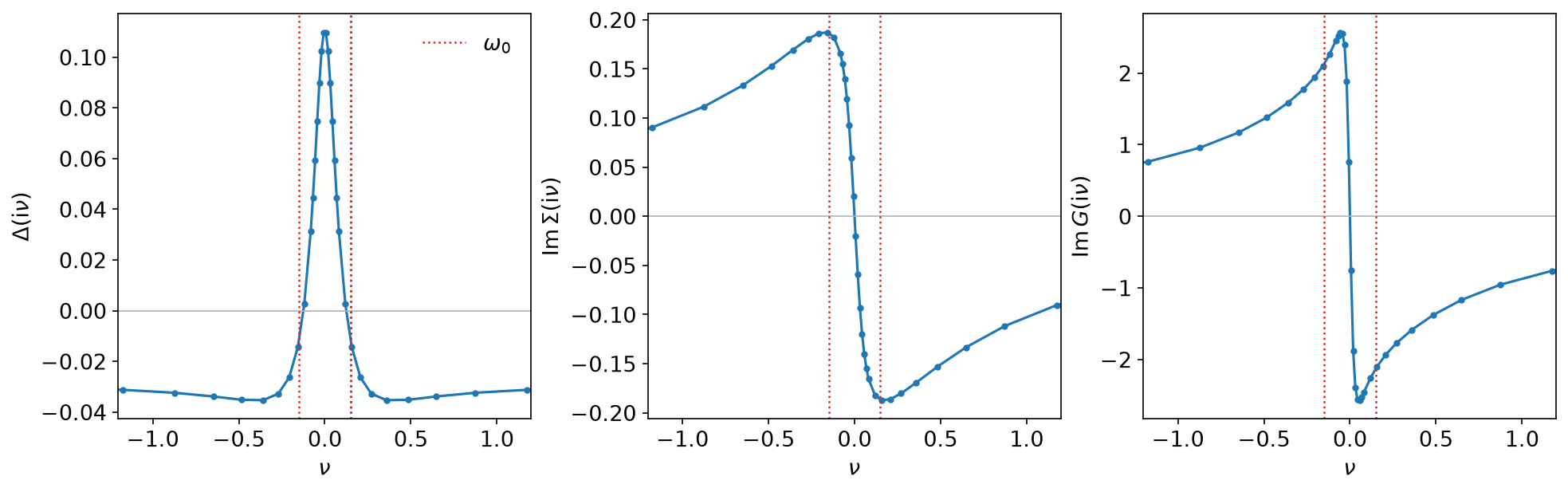
The gap is \(\Delta(\mathrm{i}\pi T) = 0.1098\), comfortably above \(\omega_0/2\), and it does not simply decay: it crosses zero just outside \(\pm\omega_0\) (the dotted lines) and reaches \(-0.0353\) before flattening out at \(-0.0292\). That negative tail is the Coulomb pseudopotential mechanism — the repulsion is pushed up to frequencies where the phonon no longer helps, and the low-frequency gap is left positive.
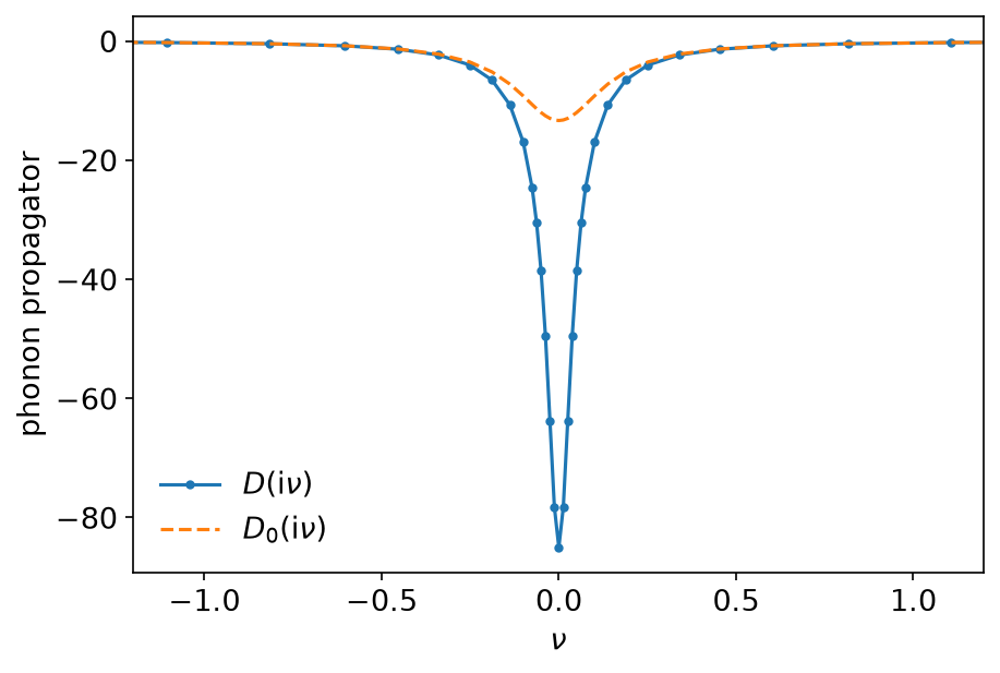
The phonon the electrons hand back is much softer than the one they were given: \(\mathcal{D}(0) = -85.0\) against a bare \(\mathcal{D}_0(0) = -2/\omega_0 = -13.3\), a factor of 6.4. For bosonic frequencies \(|\omega| \gtrsim 2\omega_0\) the two are indistinguishable.
Compactness, checked
The reason all of this fits in 45 numbers is the same reason it fits in the basis at all, and the anomalous Green’s function makes the point cleanly:
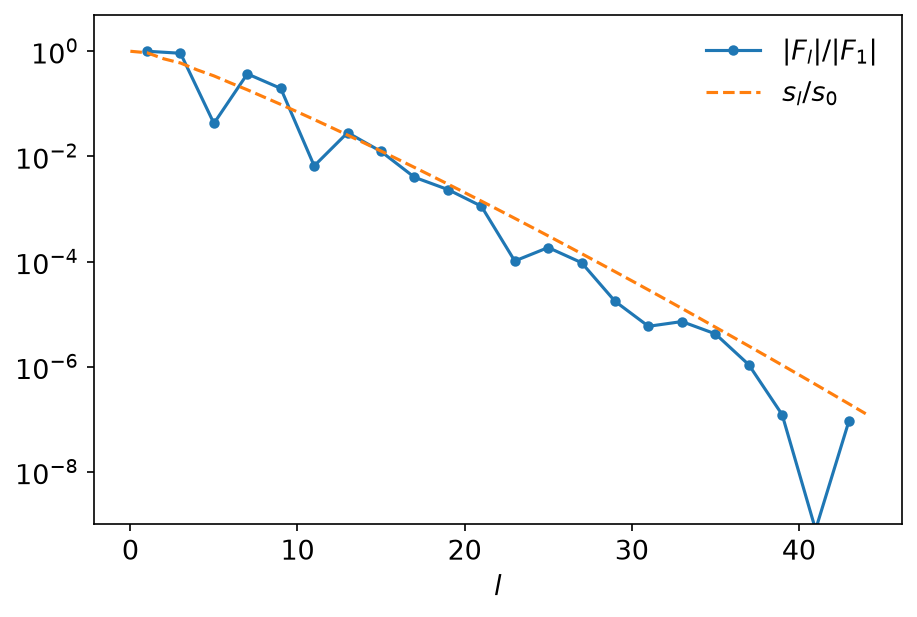
\(F\) is even in \(\nu\), so only odd \(l\) carry weight — the even coefficients sit at \(10^{-15}\), which is the round-off of the transform. What is left tracks \(s_l/s_0\) over about seven orders of magnitude (down to \(1.3\times10^{-7}\)) and stops where the expansion was truncated. A Matsubara sum reaching \(\nu = \pm 34.7\), which is where the sampling frequencies end, would have needed thousands of points to say the same thing.
The specific heat across the transition
The internal energy is a sum of three Matsubara sums, two fermionic and one
bosonic. In the basis each is a fit followed by one evaluation at
\(\tau = 0\), the same trick the TPSC sum rules use; the constant that the
basis cannot represent (\(\mathrm{i}\nu G \to 1\)) is subtracted before the
fit. Which side of \(\tau = 0\) is meant needs care. The textbook
convergence factor \(e^{\mathrm{i}\nu 0^+}\) selects \(\tau \to 0^-\), but
evaluate_tau(&[0.0]) reads \(+0.0\) as \(\tau = 0^+\), so the program
computes the \(0^+\) value. The two differ by the \(1/\mathrm{i}\nu\)
coefficient of the fitted function, and in this model that coefficient
vanishes (\(\mu = 0\), a symmetric \(\rho\), and \(\Sigma \to 0\) at large
\(\nu\)): evaluating at \(-0.0\), which the library reads as \(0^-\),
changes the two fermionic sums by about \(10^{-14}\). Away from half filling
the \(0^-\) side would have to be requested explicitly. The bosonic phonon
term is continuous at \(\tau = 0\); following the notebook, it is read at the
smallest positive sampling time \(\tau_0\).
The temperature derivative of the internal energy is the specific heat, so
eliashberg_holstein_scan solves the model twice at each of ten
temperatures — at \(T\) and at \(T + 10^{-5}\) — and takes the difference
quotient. At the stronger coupling \(\lambda_0 = 0.175\) the transition
falls inside \(T \in [0.009, 0.013]\).
The sweep holds \(\Lambda = \beta\omega_\mathrm{max} = 555.6\) fixed, so one expansion serves all twenty solves and the basis stays 36 functions throughout — which is what makes it safe to start each solve from the solution before it:
    let lambda_ir = WMAX / T_MIN;
    let (kernel, sve) = sve_for(1.0 / T_MIN, lambda_ir * T_MIN, EPS)?;
// ...
    for &temperature in &temperatures {
        let beta = 1.0 / temperature;
        let bases = Bases::from_sve(kernel, sve.clone(), beta, EPS)?;
        // ... start from the previous Σ and Δ ...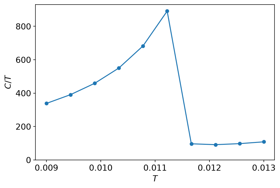
\(C/T\) climbs from 338 at \(T = 0.009\) to 891 at \(T = 0.011222\) and then falls off a cliff, to 96.7 one step later: the superconducting transition sits between those two temperatures. Above it \(C/T\) is flat and small, which is the normal state of a weakly coupled metal. The approach to the transition is also where the loop works hardest — 4476 iterations at the last superconducting point, against a dozen well above \(T_c\), the usual critical slowing down of a self-consistent solver.
Beyond the imaginary axis
The gap function here is known only at the sampling frequencies. The real-frequency gap \(\Delta(\omega)\) and the density of states of the superconductor need analytic continuation: see analytic continuation, sparse modeling and MiniPole. The DLR gives a pole representation of the same functions on the imaginary axis.
Running it
From docs/tutorial-code:
$ cargo run --profile ci --bin eliashberg_holstein
$ cargo run --profile ci --bin eliashberg_holstein_scan
$ uv run --project ../plotting python ../plotting/eliashberg_holstein_plot.py
eliashberg_holstein is one solve and takes well under a second;
eliashberg_holstein_scan is twenty solves, several of them slow, and takes a
couple of seconds. The starting self-energy is read from a committed noise
file rather than drawn at random, so that the Rust program and the Python
notebook start from the same numbers and the repository’s checks can compare
them.
Key API pieces
From sparse-ir:
| What you want | What to call |
|---|---|
| both statistics from one expansion | compute_sve, then FiniteTempBasis::from_sve_result for Fermionic and Bosonic |
| \(u^F_l(0^+)\) for a Matsubara sum | Basis::evaluate_tau(&[0.0]) (\(+0.0\) means \(0^+\), \(-0.0\) means \(0^-\)) |
| fits and evaluations at the sampling points | TauSampling, MatsubaraSampling (wrapped by IrMesh) |
From the tutorial crate (docs/tutorial-code/src):
| What you want | Tutorial helper |
|---|---|
| both bases and meshes from one expansion | Bases::new, or sve_for then Bases::from_sve |
| one pass of the loop | IrMesh::wn_to_tau, multiply, IrMesh::tau_to_wn |
| \(G(\beta - \tau) = -G(-\tau)\) on the sampling grid | IrMesh::reverse_tau |
| a Matsubara sum through the basis | IrMesh::wn_to_l, then evaluate_rows with \(u^F_l(0^+)\) |
| an integral over a density of states | gauss_legendre from tutorial::quad |
| the same basis at every temperature | fix \(\Lambda\) and vary \(\beta\) |