Fluctuation exchange
Ported from the Python notebook
FLEX_py.ipynb
of the sparse-ir tutorials,
whose author is Niklas Witt. The programs that produced every number and
figure on this page are docs/tutorial-code/src/bin/flex.rs and
docs/tutorial-code/src/bin/flex_scan.rs; the solver is in
docs/tutorial-code/src/flex.rs, and the code below is included from there.
The previous page fixed its vertices by solving two scalar equations and never iterated. The fluctuation-exchange approximation goes the other way: the interaction stays the bare \(U\), and everything is decided by a Dyson loop that is run until the self-energy stops moving. What makes it belong here is that each pass of that loop is a handful of products in \((\tau, r)\) with basis transforms between them — the frequency dependence never appears as a truncated sum.
One loop, four transforms
FLEX sums the particle-hole bubble and ladder series, which in a single band collapses to a self-energy built from the same irreducible \(\chi^0\) as on the TPSC page, dressed twice:
\[ \chi_\mathrm{sp} = \frac{\chi^0}{1 - U\chi^0}, \qquad \chi_\mathrm{ch} = \frac{\chi^0}{1 + U\chi^0}, \qquad V = U^2\left(\tfrac32 \chi_\mathrm{sp} + \tfrac12 \chi_\mathrm{ch} - \chi^0\right), \]
\[ \Sigma(\tau, r) = V(\tau, r), G(\tau, r), \qquad G(\mathrm{i}\nu, k) = \bigl[\mathrm{i}\nu - (\varepsilon_k - \mu) - \Sigma(\mathrm{i}\nu, k)\bigr]^{-1}. \]
Here \(\mathrm{i}\omega\) is a bosonic and \(\mathrm{i}\nu\) a fermionic Matsubara frequency, as in the conventions. Read as code, one step is: dress \(\chi^0\) in \((\mathrm{i}\omega, q)\), carry \(V\) to \((\tau, r)\), multiply by \(G(\tau, r)\), carry the product back to \((\mathrm{i}\nu, k)\).
        let v: Vec<Complex64> = (0..self.ckio.len())
            .map(|i| u * u * (1.5 * self.chi_spin[i] + 0.5 * self.chi_charge[i] - self.ckio[i]))
            .collect();
        let in_real_space = self.lattice.grid().k_to_r(&v);
        Ok(self.lattice.mesh_b().wn_to_tau(&in_real_space, nk)?)

        let product: Vec<Complex64> = interaction
            .iter()
            .zip(&self.grit)
            .map(|(v, g)| v * g)
            .collect();
        let in_momentum = self.lattice.grid().r_to_k(&product);
        Ok(self.lattice.mesh_f().tau_to_wn(&in_momentum, nk)?)
The bosonic mesh fits the interaction and the fermionic one fits the self-energy, on the same \(\tau\) grid — the point the TPSC page already relied on. The two grids coincide because the logistic kernel gives both statistics the same \(u_l(\tau)\); sharing one SVE between them only saves the second expansion.
Written in full, \(V\) would also carry the first-order term, a bare instantaneous \(U\) (a \(\delta(\tau)\) term). It is left out: it is frequency independent, so the basis is the wrong tool for it, and in \(\Sigma\) it would be the Hartree shift \(Un/2\), which in a single band is a shift of the chemical potential, refitted at every step anyway. That omission comes back in the gap equation below.
Keeping the denominator positive
Nothing forces \(1 - U\chi^0\) to stay positive along the way to the fixed point, and \(\chi^0\) evaluated on the non-interacting Green’s function is the largest it will ever be. At \(U = 4\) the starting point does violate it, so the interaction is walked up instead of being switched on at once:
        while target * self.max_chi() >= 1.0 {
            self.renormalisation_steps += 1;
            self.u = target / (self.max_chi() * target + 0.01);
            self.step()?;
            self.u = target;
            if self.renormalisation_steps == self.settings.renormalisation_iterations {
                break;
            }
        }
Each pass runs one FLEX step at the largest interaction the current
\(\chi^0\) can carry, which shrinks \(\chi^0\); the target \(U\) is then
retried. The loop is capped, because there is no guarantee it ever succeeds:
a genuinely ordered system has no FLEX solution to walk towards. At
\(T = 0.1\) six passes are enough; the number is written out as
renormalisation_steps.
One solve at U = 4
flex takes a \(24 \times 24\) lattice at \(\beta = 10\), filling
\(n = 0.85\), \(U = 4\), \(\varepsilon = 10^{-10}\) and a linear mixing
of \(0.2\), and runs 30 steps. The basis has 30 functions for each
statistics: 30 \(\tau\) points, 30 fermionic and 31 bosonic frequencies. The
relative movement of \(\Sigma\) in the last step is \(1.3\times10^{-5}\),
and \(\mu = -0.6713\).
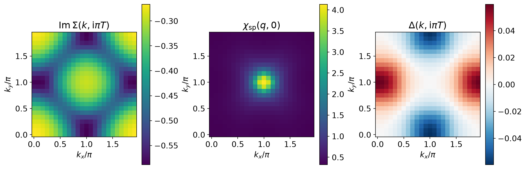
\(|\mathrm{Im},\Sigma|\) is largest at the antinodes \((\pi, 0)\) and smallest along the diagonal — the momentum-selective scattering that opens a pseudogap — and \(\chi_\mathrm{sp}\) is piled up at \(M = (\pi, \pi)\), enhanced there by a factor of \(17.5\) over \(\chi^0\) against \(2.3\) at \(\Gamma\).
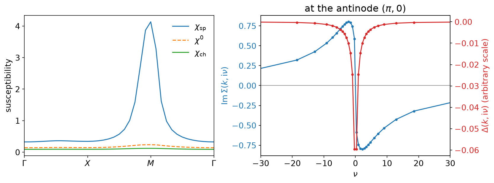
Against frequency, \(\mathrm{Im},\Sigma\) is odd, largest in magnitude at the first Matsubara frequency and decaying from there; the run gives \(\mathrm{Im},\Sigma(\mathrm{i}\pi T, (\pi,0)) = -0.588\). Its sign, opposite to that of \(\nu\) at every sampling frequency, is the statement that the solution is causal.
The linearised gap equation
With the fluctuations in hand, the question is whether they pair. The linearised Eliashberg equation
\[ \lambda, \Delta(\mathrm{i}\nu, k) = \frac{T}{N_k} \sum_{\mathrm{i}\nu’, k’} V^S(\mathrm{i}\nu - \mathrm{i}\nu’, k - k’), F(\mathrm{i}\nu’, k’), \qquad F = -|G|^2,\Delta, \]
is an eigenvalue problem whose leading \(\lambda\) reaches 1 at \(T_\mathrm{c}\). (The sign is carried by \(F\), as in the code; writing \(F = |G|^2\Delta\) with a minus sign in front of the sum is the same equation.) The convolution is a plain product \(V^S(\tau, r)F(\tau, r)\). The singlet vertex is not the one in the self-energy: the charge fluctuations enter with the opposite sign, \(V^S = U + U^2\left(\tfrac32\chi_\mathrm{sp} - \tfrac12\chi_\mathrm{ch}\right)\), of which the code keeps the frequency-dependent part. Applying it is the same four transforms as one FLEX step, so the power method costs about what a few self-consistency steps cost, seeded with a \(d_{x^2-y^2}\) gap \(\cos k_x - \cos k_y\).
Here the dropped bare \(U\) (the \(\delta(\tau)\) term of \(V^S\)) matters. It contributes exactly zero in the \(d\)-wave channel, because such a gap sums to zero over the zone, but not outside it, and without it the operator has a spurious mode whose eigenvalue is \(-1.28\) — larger in magnitude than \(\lambda_d\). The seed has almost no overlap with it, so the iterate sits on the \(d\)-wave answer for tens of steps and then leaves it. A fixed step count would land right at that crossover; the loop therefore stops when \(\lambda\) moves by less than \(10^{-4}\), which happens after 8 steps with three orders of magnitude to spare. The step count is written out too.
The result is \(\lambda_d = 0.4568\) at \(T = 0.1\): the right symmetry, well short of the transition. The gap in the third panel above changes sign under \(k_x \leftrightarrow k_y\) and vanishes on the zone diagonal; the eigenvector’s overall scale means nothing, only its shape does.
(The \(\lambda\) here is an eigenvalue of the gap equation. It is unrelated to the electron-phonon coupling \(\lambda_0\) of the Eliashberg page.)
Cooling towards T_c
flex_scan repeats the calculation on a \(64 \times 64\) lattice at seven
temperatures from \(T = 0.08\) down to \(0.025\), with
\(\Lambda = \beta\omega_\mathrm{max}\) held at \(10^3\) and
\(\varepsilon = 10^{-8}\). Holding \(\Lambda\) fixed means one SVE serves
every temperature —
    let beta_init = 1.0 / TEMPERATURES[0];
    let (kernel, sve) = sve_for(beta_init, LAMBDA / beta_init, EPS)?;
// ...
    for (index, &temperature) in TEMPERATURES.iter().enumerate() {
        let beta = 1.0 / temperature;
        let lattice = Lattice::from_sve(kernel, sve.clone(), NK_LIN, NK_LIN, T_HOP, beta, EPS)?;
— and that every temperature has a basis of the same 43 functions, which in turn is what makes it legal to carry the converged \(\Sigma\) of one temperature into the next as a starting point. With that head start, the renormalisation loop runs only at the first temperature (nine passes) and never again.
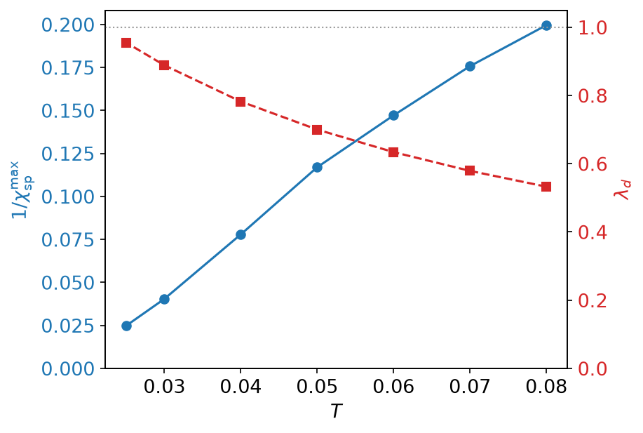
\(1/\chi_\mathrm{sp}^{\max}\) falls almost linearly — the Curie–Weiss form — from \(0.1996\) to \(0.0248\), extrapolating to zero near \(T \approx 0.019\), while \(\lambda_d\) climbs from \(0.533\) to \(0.955\) and would reach 1 at about \(T \approx 0.021\). The two temperatures are close because in this approximation it is the spin fluctuations that do the pairing: the gap equation is driven by the same \(\chi_\mathrm{sp}\) that is diverging.
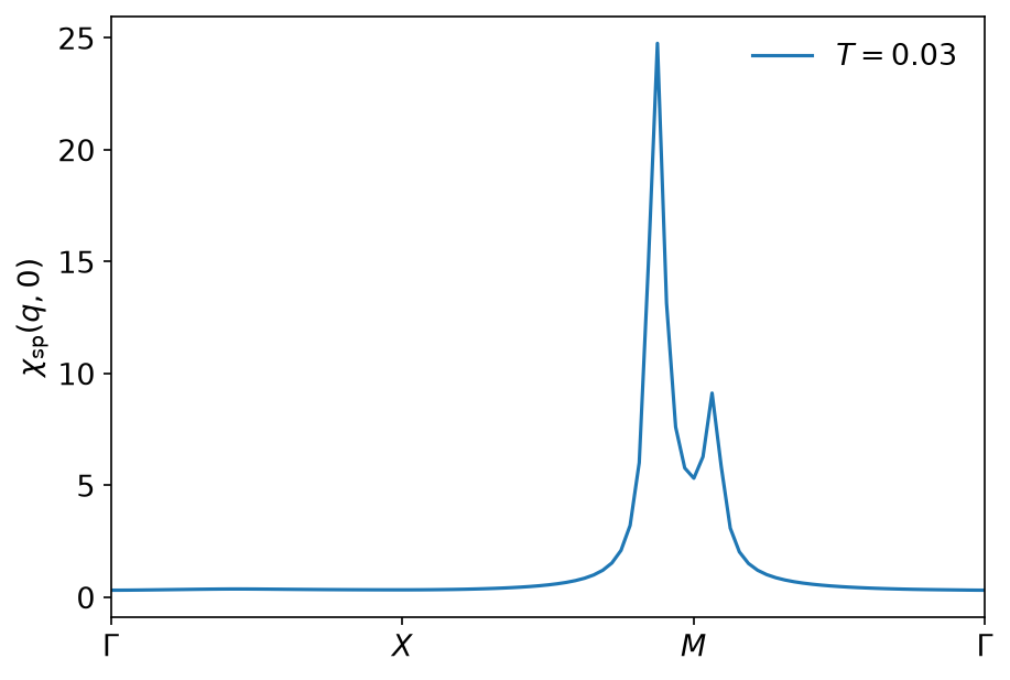
The finer grid also resolves what the \(24\times24\) run could not: at \(n = 0.85\) the peak is not at \(M\). Nesting is incommensurate, and \(\chi_\mathrm{sp}\) peaks at \((\pi, 7\pi/8)\) with the value \(24.8\) against \(5.3\) at \(M\) itself — a factor of nearly five that a commensurate grid would have missed entirely.
Beyond the imaginary axis
FLEX gives \(\Sigma\), \(\chi\) and \(\Delta\) on the sampling frequencies only. To look at the pseudogap or the gap on the real axis, the same data have to be continued: see analytic continuation, sparse modeling and MiniPole. The DLR gives a pole representation of the same functions on the imaginary axis.
Running it
From docs/tutorial-code:
$ cargo run --profile ci --bin flex
$ cargo run --profile ci --bin flex_scan
$ uv run --project ../plotting python ../plotting/flex_plot.py
flex is one solve and takes under half a second; flex_scan is seven solves
on a grid seven times larger and takes a few seconds. The repository’s checks
compare the outputs with the Python notebook, including the
renormalisation-pass and power-method step counts, the sign of
\(\mathrm{Im},\Sigma\) at every frequency, and the symmetry of the gap.
Key API pieces
From sparse-ir:
| What you want | What to call |
|---|---|
| one SVE reused across temperatures | compute_sve with LogisticKernel::new(Λ), then FiniteTempBasis::from_sve_result per \(\beta\) |
| \(u^F_l(0^+)\) for the filling | Basis::evaluate_tau(&[0.0]) (\(+0.0\) means \(0^+\)) |
| fits and evaluations at the sampling points | TauSampling, MatsubaraSampling (wrapped by IrMesh) |
From the tutorial crate (docs/tutorial-code/src):
| What you want | Tutorial helper |
|---|---|
| one step of a Dyson loop | IrMesh::wn_to_tau, MomentumGrid::k_to_r, multiply, MomentumGrid::r_to_k, IrMesh::tau_to_wn |
| \(\chi^0\) as a real-space product | IrMesh::reverse_tau, then the bosonic IrMesh::tau_to_wn |
| the filling \(n = 2[1 + G(\tau = 0^+)]\) | IrMesh::wn_to_l, then evaluate_rows with \(u^F_l(0^+)\) |
| the chemical potential at fixed \(n\) | brent from tutorial::roots |
| one SVE reused across temperatures | sve_for, then Lattice::from_sve per \(\beta\) |
| a whole basis at fixed \(\Lambda\) | keep \(\beta\omega_\mathrm{max}\) constant and vary \(\beta\) |