Introduction
sparse-ir compresses the imaginary-time Green’s functions of finite-temperature
many-body theory. A Green’s function on a dense grid in imaginary time or
Matsubara frequency carries far fewer independent numbers than grid points, and
the library provides three ways to exploit that:
- The intermediate representation (IR) basis. An orthonormal basis obtained from a singular value expansion of the analytic-continuation kernel. Its size grows only logarithmically with the cutoff \(\Lambda = \beta\omega_\mathrm{max}\), and a matching set of sparse sampling points in \(\tau\) and in Matsubara frequency is enough to recover the expansion. See Sparse sampling and Transformation from and to IR.
- The discrete Lehmann representation (DLR). A sum of simple poles on a fixed real-frequency grid, chosen by an interpolative decomposition of the kernel. It needs no IR basis, comes with its own sampling nodes, and can also be built from an existing IR basis. See Discrete Lehmann representation.
- MiniPole. A data-adapted compression: ESPRIT extracts a handful of complex poles from one particular function, which also gives an analytic continuation. See MiniPole.
The IR basis and the DLR are fixed representations shared by every function with the same \(\beta\), \(\omega_\mathrm{max}\) and accuracy; MiniPole adapts to the data. For how the three are related, where each came from and what each is convenient for, see IR, DLR and MiniPole: history and comparison on the theory site.
How this book is organised
Getting started covers installation and the conventions used throughout, including the Matsubara-frequency index; read Conventions before comparing numbers with another code. Representations introduces the IR basis, the DLR and MiniPole. Analytic continuation goes from imaginary-time data back to real frequency. Applied examples solve complete many-body problems with the IR basis.
Most pages follow a notebook of the Python and Julia tutorials, sparse-ir-tutorial; each page says which one.
How this book is built
The Rust code on these pages is included from the example programs in
docs/tutorial-code/ rather than copied by hand, so it is the code that is
actually compiled and run, and every figure was drawn from numbers those
programs wrote. Most examples are checked against reference values from the
Python implementation; the rest, such as the IR-independent DLR and MiniPole,
check themselves against closed-form results. Each page ends with the command that reproduces it; run
it from docs/tutorial-code.
Installation
sparse-ir requires Rust 1.96 or newer. Add it from crates.io:
[dependencies]
sparse-ir = "0.13.0"
This book is written against sparse-ir 0.13. The sparse-ir crate re-exports
everything the book uses; it is built from four crates you can also depend on
directly: sparse-ir-core (statistics, sampling, fitting), sparse-ir-basis
(kernels, SVE and the IR basis), sparse-ir-dlr (the DLR) and
sparse-ir-minipole (ESPRIT and MiniPole). To follow the development branch
instead, use the Git dependency, pinned to a tested rev for reproducible
projects:
[dependencies]
sparse-ir = { git = "https://github.com/SpM-lab/sparse-ir-rs", branch = "main" }
sparse-ir is pure Rust and needs no system libraries: its linear algebra goes
through faer by default. If you
would rather route the matrix products through the LP64 BLAS already installed
on your machine, turn on the system-blas feature:
[dependencies]
sparse-ir = { version = "0.13.0", features = ["system-blas"] }
Both backends compute the same numbers; the feature only changes which implementation multiplies the matrices.
The API reference is at
docs.rs/sparse-ir for the release and
here for
main.
Conventions
This page fixes the notation and the conventions used throughout the book. They are the ones that most often differ between codes, so read it before comparing numbers with another library.
Notation
| Symbol | Meaning |
|---|---|
| \(\beta\), \(\omega_\mathrm{max}\), \(\Lambda = \beta\omega_\mathrm{max}\) | inverse temperature, frequency cutoff, dimensionless cutoff |
| \(\tau\) | imaginary time, \(\tau \in [0, \beta)\) |
| \(\omega\) | real frequency |
| \(\mathrm{i}\nu_n = \mathrm{i}n\pi/\beta\) | Matsubara frequency with the reduced index \(n\) (see below) |
| \(\mathrm{i}\nu\), \(\mathrm{i}\omega\) | fermionic and bosonic Matsubara frequencies, when one formula has both |
| \(m\) | textbook Matsubara index, \(n = 2m + \zeta\) |
| \(\zeta\) | \(1\) for fermions, \(0\) for bosons |
| \(u_l(\tau)\), \(\hat u_l(\mathrm{i}\nu)\), \(v_l(\omega)\), \(s_l\) | IR basis functions and singular values, \(l = 0, \dots, L-1\) (basis.u, basis.uhat, basis.v, basis.s) |
| \(g_l\) | IR expansion coefficients |
| \(\omega_p\), \(c_p\) | DLR poles and coefficients |
| \(\varepsilon\) | accuracy parameter of a representation (see below) |
Three representations, one accuracy parameter
sparse-ir provides three compact representations of a Green’s function. Each
is built from \(\beta\), \(\omega_\mathrm{max}\) and an accuracy
\(\varepsilon\), but \(\varepsilon\) means something different for each:
| Representation | Built by | \(\varepsilon\) means |
|---|---|---|
| IR basis (sparse sampling) | FiniteTempBasis::new(LogisticKernel::new(beta * wmax)?, beta, Some(eps), None) | singular-value cutoff: keep \(l\) with \(s_l/s_0 > \varepsilon\) |
| DLR (discrete Lehmann representation) | DiscreteLehmannRepresentation::new(beta, wmax, eps) | pivot tolerance of the interpolative decomposition that selects the poles |
| MiniPole (MiniPole) | mini_pole_dlr_from(&dlr, &coeffs, ¶ms) | ESPRIT tolerance err; it controls how many poles are kept and is not a bound on the reconstruction error |
The IR basis and the DLR are fixed, data-independent representations: build them once for given \(\beta\), \(\omega_\mathrm{max}\) and \(\varepsilon\), and expand any Green’s function in them. MiniPole is data-adapted: it compresses one particular function into a few poles, which may lie off the real axis.
Imaginary time runs over [0, β), but the sampling times do not
Green’s functions are functions of \(\tau \in [0, \beta)\), and that is the domain the basis functions \(u_l(\tau)\) are defined on.
The sampling times, however, are reported on the symmetric interval
\([-\beta/2, \beta/2]\). sparse-ir picks them as the roots of the first
discarded basis function \(u_L\) and then folds each one that landed beyond
\(\beta/2\) down by \(\beta\), which for a fermionic function means flipping
its sign as well:
G(τ − β) = −G(τ) (fermionic), G(τ − β) = +G(τ) (bosonic).
The folding is not cosmetic. Near \(\tau = \beta\) the values of \(G\) are tiny and their relative accuracy is poor; the reflected point near \(\tau = 0\) carries the same information with far more significant digits. Everything that takes a \(\tau\) accepts the whole range \([-\beta, \beta]\) and applies the relation above, so you can hand it either form. If you compare sampling points with another library, compare them after folding.
Statistics is part of the type
A basis is fermionic or bosonic, and which one it is shows up in the type, not in a runtime flag:
use sparse_ir::{Fermionic, FiniteTempBasis, LogisticKernel};

let (beta, wmax, eps) = (10.0, 1.0, 1e-10);
let kernel = LogisticKernel::new(beta * wmax).unwrap();
let basis =
    FiniteTempBasis::<LogisticKernel, Fermionic>::new(kernel, beta, Some(eps), None).unwrap();
assert!(basis.size() > 0);
Matsubara frequencies: the reduced index
A Matsubara frequency is stored as one integer \(n\), the MatsubaraFreq
type (FermionicFreq, BosonicFreq), with
\[ \nu_n = \frac{n\pi}{\beta}, \qquad n \text{ odd for fermions } (\pm1, \pm3, \dots), \quad n \text{ even for bosons } (0, \pm2, \dots). \]
This \(n\) is the reduced index. It is not the textbook index \(m\)
of \(\nu = (2m + \zeta)\pi/\beta\); the two are related by
\(n = 2m + \zeta\). The lowest positive fermionic frequency \(\pi/\beta\)
is therefore FermionicFreq::new(1), and a fermionic n = 0 or a bosonic
n = 1 is rejected:
use sparse_ir::{BosonicFreq, FermionicFreq};
use std::f64::consts::PI;

let beta = 10.0;
assert!((FermionicFreq::new(1).unwrap().value(beta) - PI / beta).abs() < 1e-15);
assert!((BosonicFreq::new(2).unwrap().value(beta) - 2.0 * PI / beta).abs() < 1e-15);
assert!(FermionicFreq::new(0).is_err());
assert!(BosonicFreq::new(1).is_err());
Every integer the library hands you, such as the points returned by
MatsubaraSampling::sampling_points(), is a reduced index. If you index an
array by \(m = 0, 1, 2, \dots\), convert with \(m = (n - \zeta)/2\).
One place uses a different convention. The MiniPole entry points that start
from a DLR (mini_pole_dlr_from, mini_pole_dlr) evaluate the function on the
contour \(\omega_n = (2n+1)\pi/\beta\) with a contour index \(n\), and
they do so even for a bosonic DLR. The MiniPole
page explains why.
Nothing is computed twice by accident
Constructing a FiniteTempBasis runs a singular value expansion (SVE), which
is by far the most expensive step in the library. The SVE depends only on the
kernel (through \(\Lambda\)) and on \(\varepsilon\). If you need a
fermionic and a bosonic basis for the same \(\Lambda\), compute the expansion
once and build both bases from it with FiniteTempBasis::from_sve_result:
use sparse_ir::{compute_sve, Bosonic, Fermionic, FiniteTempBasis, LogisticKernel, TworkType};

let (beta, wmax, eps) = (10.0, 1.0, 1e-10);
let kernel = LogisticKernel::new(beta * wmax).unwrap();
let sve = compute_sve(kernel, Some(eps), None, None, TworkType::Auto).unwrap();
let fermionic = FiniteTempBasis::<LogisticKernel, Fermionic>::from_sve_result(
    kernel, beta, sve.clone(), Some(eps), None,
)
.unwrap();
let bosonic =
    FiniteTempBasis::<LogisticKernel, Bosonic>::from_sve_result(kernel, beta, sve, Some(eps), None)
        .unwrap();
assert_eq!(fermionic.size(), bosonic.size());
The two bases share their singular values and functions; only the statistics of \(\hat u_l(\mathrm{i}\nu)\) differs.
Sparse sampling
Ported from the Python notebook
sparse_sampling_demo_py.ipynb
of the sparse-ir tutorials.
The program that produced every number and figure on this page is
docs/tutorial-code/src/bin/sparse_sampling_demo.rs.
This page shows how to infer the IR expansion coefficients of a Green’s function from its values at a handful of points. This is the sparse sampling technique that makes the basis useful in practice: you never need \(G\) on a dense grid, only at as many points as the basis has functions.
Setup
Take the semicircular spectral function of full bandwidth 2,
\[ \rho(\omega) = \frac{2}{\pi}\sqrt{1-\omega^2}, \]
at \(\beta = 10^4\) and \(\omega_\mathrm{max} = 1\). Asking for \(\varepsilon = 10^{-15}\) gives a basis of 104 functions.
use num_complex::Complex64;
use sparse_ir::{Fermionic, FiniteTempBasis, LogisticKernel, MatsubaraSampling, TauSampling};
/// Inverse temperature. Large enough that the basis is interesting (a few tens
/// of functions) while `ωmax = 1` keeps the spectral function simple.
const BETA: f64 = 10_000.0;
const WMAX: f64 = 1.0;
const EPS: f64 = 1e-15;
    let kernel = LogisticKernel::new(BETA * WMAX)?;
    let basis = FiniteTempBasis::<LogisticKernel, Fermionic>::new(kernel, BETA, Some(EPS), None)?;
Ok::<(), Box<dyn std::error::Error>>(())
The exact coefficients are \(g_l = -s_l \rho_l\) with \(\rho_l = \int \mathrm{d}\omega, v_l(\omega) \rho(\omega)\). They fall off exponentially, which is the whole reason the basis is small:
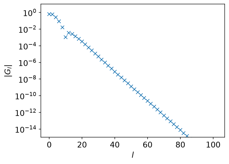
Only even \(l\) is shown: \(\rho\) is even in \(\omega\), so every odd coefficient vanishes.
From the sampling times
TauSampling picks the default sampling times, the roots of the first basis
function the truncation discarded, and builds the matrix
\(A_{il} = u_l(\tau_i)\) that turns coefficients into values. evaluate
goes from coefficients to values, fit the other way:
    let tau_sampling = TauSampling::<Fermionic>::new(&basis)?;
    let tau_points = tau_sampling.sampling_points().to_vec();
    // The default sampling times are folded around β/2, so they are reported
    // on the symmetric interval rather than on [0, β). See the conventions
    // page of the book.
    assert!(
        tau_points
            .iter()
            .all(|&tau| (-BETA / 2.0..=BETA / 2.0).contains(&tau)),
        "the default sampling times must lie in [-β/2, β/2]"
    );
    let g_tau = tau_sampling.evaluate(&g_l)?; // coefficients -> values
    let g_l_from_tau = tau_sampling.fit(&g_tau)?; // values -> coefficients
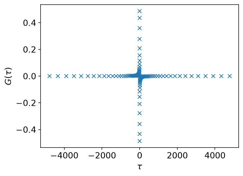
There are 104 sampling times, as many as the basis has functions, and the
condition number (condition_number) is about 51.8. A fit from the sampling
times therefore loses one or two significant digits, no more.
The times come back on \([-\beta/2, \beta/2]\) rather than on \([0, \beta)\); see Conventions for why.
From the sampling frequencies
MatsubaraSampling does the same in frequency. Its points are MatsubaraFreq
values, and n() returns the reduced index \(n\) of
\(\mathrm{i}\nu_n = \mathrm{i}n\pi/\beta\). For fermions \(n\) is odd
(\(n = 2m + 1\) in terms of the textbook index \(m\)), so
FermionicFreq::new(1) is \(\nu = \pi/\beta\) and FermionicFreq::new(0) is
an error; see
Conventions.
\(G\) is complex there, so the coefficients go in and come back as
Complex64:
    let matsubara_sampling = MatsubaraSampling::<Fermionic>::new(&basis)?;
    // The points are MatsubaraFreq values; n() is the reduced index n of
    // iν_n = i n π/β, which is odd for fermions.
    let matsubara_points: Vec<i64> = matsubara_sampling
        .sampling_points()
        .iter()
        .map(|freq| freq.n())
        .collect();
    assert!(
        matsubara_points.iter().all(|n| n % 2 != 0),
        "fermionic Matsubara indices must be odd"
    );
    // G(iν) is complex, so the coefficients go in, and come back, as Complex64.
    let g_l_complex: Vec<Complex64> = g_l.iter().map(|&g| Complex64::new(g, 0.0)).collect();
    let g_iv = matsubara_sampling.evaluate(&g_l_complex)?;
    let g_l_from_matsubara: Vec<f64> = matsubara_sampling
        .fit(&g_iv)?
        .iter()
        .map(|c| c.re)
        .collect();
The coefficients here are real, so the complex copy is not needed:
evaluate_real takes real coefficients and returns complex values, and
fit_real fits real coefficients to complex values.
The condition number is about 213, roughly four times that of the sampling times. That is the price of working in frequency.
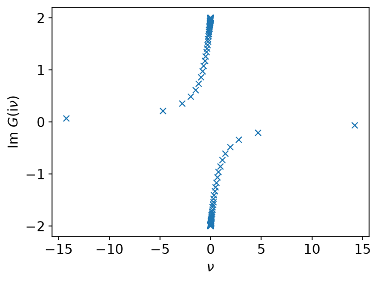
Because \(\rho\) is even in \(\omega\), \(G(\mathrm{i}\nu)\) is purely imaginary; the real part that comes back is rounding error, about \(10^{-15}\) of the imaginary part.
Comparison with the exact result
Both fits recover the exact coefficients:
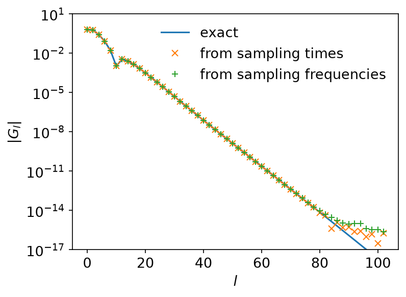
The curves lie on top of each other until the coefficients themselves drop below \(10^{-14}\), where there is nothing left to recover. The differences say the same thing more directly:
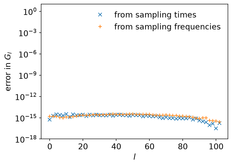
The error sits at \(10^{-16}\)–\(10^{-15}\). The accuracy of the basis times the condition number of the fit bounds it by about \(10^{-15} \times 52 \approx 5 \times 10^{-14}\) from the sampling times and \(10^{-15} \times 213 \approx 2 \times 10^{-13}\) from the sampling frequencies, so both fits are well within the bound.
Key API pieces
| What you want | What to call |
|---|---|
| the sampling points | TauSampling::sampling_points, MatsubaraSampling::sampling_points |
| the reduced index of a Matsubara point | MatsubaraFreq::n |
| how much a fit costs you | condition_number |
| coefficients → values | evaluate (evaluate_real for real coefficients in frequency) |
| values → coefficients | fit (fit_real for real coefficients in frequency) |
| your own points instead of the defaults | TauSampling::with_sampling_points, MatsubaraSampling::with_sampling_points |
evaluate and fit have _to variants that write into a slice you own, and
_nd variants for a whole array of Green’s functions sharing one basis. Use
those in an inner loop, where allocating per call would dominate.
The same sampling objects work on a DLR: TauSampling::new(&dlr) and
MatsubaraSampling::new(&dlr) sample at the DLR’s own nodes. See
Discrete Lehmann representation.
Running it
From docs/tutorial-code:
cargo run --profile ci --bin sparse_sampling_demo
uv run --project ../plotting python ../plotting/sparse_sampling_demo_plot.py
Transformation from and to IR
Ported from the Python notebook
transformation_py.ipynb
of the sparse-ir tutorials.
The program that produced every number and figure on this
page is docs/tutorial-code/src/bin/transformation.rs.
The basis is only useful once your data is in it. This page covers the three ways data usually arrives (as poles, as a smooth spectral function, as \(G(\tau)\) on a grid) and the way back out.
Poles
A Green’s function made of poles,
\[ G(\mathrm{i}\nu) = \sum_{p} \frac{a_p}{\mathrm{i}\nu - \omega_p}, \qquad A(\omega) = \sum_p a_p \delta(\omega - \omega_p), \]
needs no quadrature at all. The logistic kernel expands the regularized spectral function, which for bosons carries an extra factor,
\[ \rho(\omega) = \sum_p c_p \delta(\omega - \omega_p), \qquad c_p = \begin{cases} a_p & \text{(fermions)},\ a_p / \tanh(\beta\omega_p/2) & \text{(bosons)},\end{cases} \]
so the overlap integral collapses to \(\rho_l = \sum_p c_p v_l(\omega_p)\).
The example takes one bosonic pole at \(\omega_1 = 0.1\) with
\(a_1 = 1\), at \(\beta = 15\), \(\omega_\mathrm{max} = 10\) and
\(\varepsilon = 10^{-10}\), a basis of 34 functions. evaluate_omega
gives the \(v_l(\omega_p)\), and \(g_l = -s_l \rho_l\). The
DiscreteLehmannRepresentation says the same thing in one call: build it with
the poles (from_ir_with_poles), and to_ir_nd turns the DLR coefficients
\(c_p\) into IR coefficients (see
Discrete Lehmann representation).
use std::error::Error;

use sparse_ir::DlrFromIr;
use sparse_ir::{
    Basis, Bosonic, DiscreteLehmannRepresentation, Fermionic, FiniteTempBasis, LogisticKernel,
    MatsubaraSampling, TauSampling,
};
use sparse_ir::{Matrix, TypedTensor};
/// The pole section: one bosonic pole, placed just off zero so that the
/// `1/tanh(βω/2)` regularizer is large but finite.
const POLE_BETA: f64 = 15.0;
const POLE_WMAX: f64 = 10.0;
const POLE_EPS: f64 = 1e-10;
const POLE_POSITION: f64 = 0.1;
const POLE_WEIGHT: f64 = 1.0;
fn pole_basis() -> Result<FiniteTempBasis<LogisticKernel, Bosonic>, Box<dyn Error>> {
    let kernel = LogisticKernel::new(POLE_BETA * POLE_WMAX)?;
    Ok(FiniteTempBasis::<LogisticKernel, Bosonic>::new(
        kernel,
        POLE_BETA,
        Some(POLE_EPS),
        None,
    )?)
}
    let basis = pole_basis()?;

    // For the logistic kernel the bosonic spectral function carries the
    // `1/tanh(βωₚ/2)` factor, so that is what the basis expands.
    let regularized = POLE_WEIGHT / (0.5 * POLE_BETA * POLE_POSITION).tanh();

    let v_at_pole: Matrix<f64> = basis.evaluate_omega(&[POLE_POSITION])?;
    let rho_l: Vec<f64> = (0..basis.size())
        .map(|l| *v_at_pole.get(&[0, l]).unwrap() * regularized)
        .collect();
    let g_l: Vec<f64> = basis
        .s()
        .iter()
        .zip(&rho_l)
        .map(|(s, rho)| -s * rho)
        .collect();

    // The DLR says the same thing in one call: it knows how a pole maps onto
    // the basis, so it takes the DLR coefficient `cₚ = aₚ/tanh(βωₚ/2)` and
    // returns `gₗ` directly.
    let dlr =
        DiscreteLehmannRepresentation::<Bosonic>::from_ir_with_poles(&basis, vec![POLE_POSITION])?;
    let weights = TypedTensor::from_vec_col_major(vec![1], vec![regularized])?;
    let g_l_dlr = dlr.to_ir_nd::<f64>(None, &weights, 0)?;
Ok::<(), Box<dyn std::error::Error>>(())
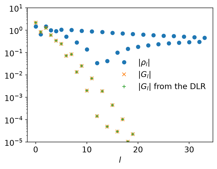
Both routes give the same coefficients:
From a smooth spectral function
For a smooth \(\rho\) the coefficients are an integral,
\[ \rho_l = \int_{-\omega_\mathrm{max}}^{\omega_\mathrm{max}} \mathrm{d}\omega, v_l(\omega), \rho(\omega). \]
A single Gauss-Legendre rule over the whole interval will not do. The roots of \(v_l\) crowd together near \(\omega = 0\), far more densely than the roots of a Legendre polynomial of the same degree, so the integrand varies on a scale the rule cannot see. Split the interval at the knots the basis functions are built on, where each \(v_l\) is a polynomial, and apply the rule on every piece; if \(\rho\) is smooth within a piece, the result converges exponentially in the order.
PiecewiseLegendrePolyVector::get_knots hands you exactly those division
points. integrate_segments is a tutorial-crate helper that applies a
Gauss-Legendre rule on every segment; sparse_ir::legendre provides such a
rule if you want to write your own.
fn overlap_with_v<F>(basis: &FiniteTempBasis<LogisticKernel, Fermionic>, f: F) -> Vec<f64>
where
    F: Fn(f64) -> f64,
{
    let v = basis.v();
    let edges = v.get_knots(None);
    let order = v.get_polyorder() + 8;
    (0..basis.size())
        .map(|l| {
            let poly = &v[l];
            integrate_segments(|omega| poly.evaluate(omega) * f(omega), &edges, order)
        })
        .collect()
}
With \(\rho_l\) in hand, \(g_l = -s_l \rho_l\).
The spectral function here is three Gaussian peaks, one of them narrow:
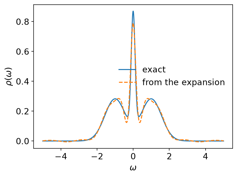
The dashed line is \(\sum_l v_l(\omega) \rho_l\), evaluated on a grid the basis never saw: the expansion is good everywhere, not only at the knots.
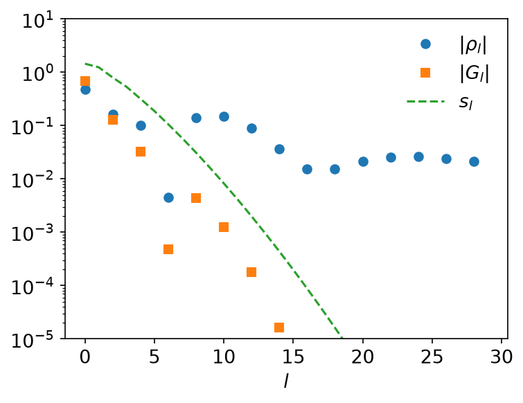
\(g_l\) falls off like \(s_l\); \(\rho_l\) does not, because the narrow peak needs high \(l\) to resolve. That is the normal picture, and the next section shows what the abnormal one looks like.
From IR to imaginary time
With \(g_l\) in hand, \(G(\tau) = \sum_l u_l(\tau) g_l\) on any grid you
like. Either evaluate the basis functions (evaluate_tau returns a
[taus.len(), basis.size()] matrix),
    // Directly: `G(τ) = Σₗ uₗ(τ) gₗ`.
    let u_at_taus: Matrix<f64> = basis.evaluate_tau(&taus)?;
    let g_tau_direct: Vec<f64> = (0..taus.len())
        .map(|i| {
            (0..basis.size())
                .map(|l| *u_at_taus.get(&[i, l]).unwrap() * g_l[l])
                .sum()
        })
        .collect();
or hand the same points to TauSampling, which builds that matrix once and
can also go back the other way:
    // Or through `TauSampling`, which builds the same matrix once and can also
    // go the other way. Any set of τ points will do — these are not the
    // default sampling times.
    let sampling = TauSampling::<Fermionic>::with_sampling_points(basis, taus.clone())?;
    let g_tau_sampling = sampling.evaluate(&g_l)?;
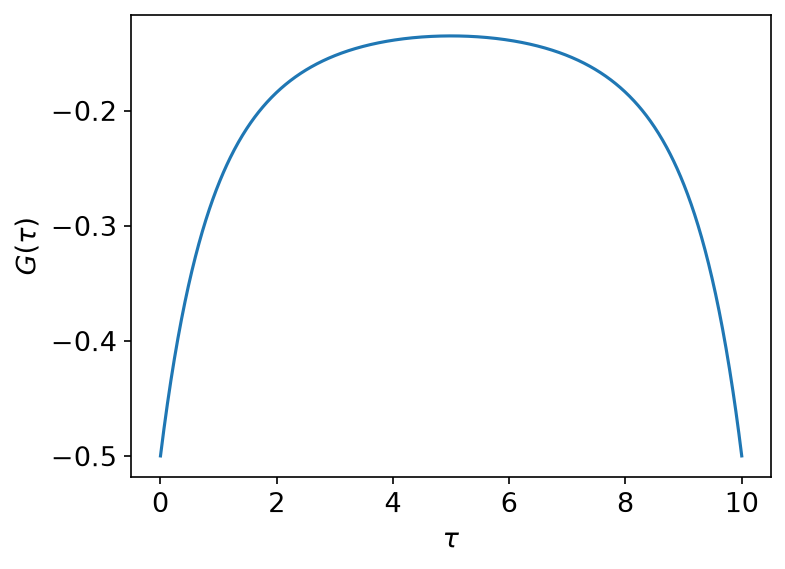
Nothing requires these to be the default sampling points. They are an arbitrary dense grid here, which is what you want for a figure:
From full imaginary-time data
Going back from \(G(\tau)\) known everywhere, the stable route is the overlap integral
\[ g_l = \int_0^\beta \mathrm{d}\tau, G(\tau), u_l(\tau), \]
by the same composite quadrature as before, now on the knots of basis.u().
It recovers the coefficients to the accuracy of the basis:
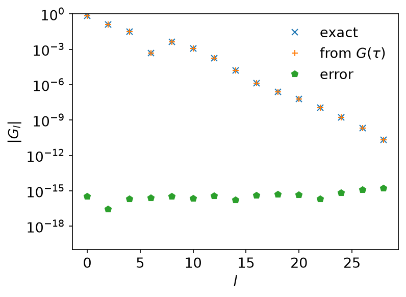
Only even \(l\) is shown: \(\rho\) is even in \(\omega\), so the odd coefficients vanish.
What if ωmax is too small?
Expand the very same \(G(\tau)\) in a basis built for \(\omega_\mathrm{max} = 0.5\), far too narrow for a spectral function that reaches out to \(\omega \approx 3\):
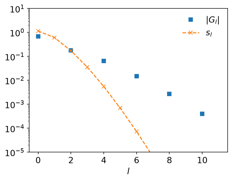
The coefficients stop following the singular values down. That is the signal, and the only one you get: nothing errors, the expansion simply does not converge. If \(g_l\) does not decay like \(s_l\), widen \(\omega_\mathrm{max}\).
Many Green’s functions at once
evaluate and fit have _nd variants that transform one axis of an array,
which is what you want when many Green’s functions share a basis: orbital
indices, momenta, a self-energy on a grid.
    // coeffs has shape [2, 3, basis.size()]; transform along axis 2.
    let sampling = MatsubaraSampling::<Fermionic>::new(basis)?;
    let values = sampling.evaluate_nd_real(None, &coeffs, 2)?;
    let recovered = sampling.fit_nd_real(None, &values, 2)?;
The _real variants take real coefficients and return complex values, which
saves you building a complex copy of an array that has no imaginary part.
Key API pieces
| What you want | What to call |
|---|---|
| \(v_l\) or \(u_l\) at your own points | Basis::evaluate_omega, Basis::evaluate_tau |
| the segments to integrate over | PiecewiseLegendrePolyVector::get_knots |
| a Gauss-Legendre rule | sparse_ir::legendre |
| DLR coefficients \(c_p\) → \(g_l\) | DiscreteLehmannRepresentation::from_ir_with_poles, to_ir_nd |
| one axis of an array | the _nd and _nd_real variants |
Tutorial-crate helper (not part of sparse-ir):
| What you want | What to call |
|---|---|
| a composite Gauss-Legendre integral over given segments | sparse_ir_tutorial::integrate_segments |
Running it
From docs/tutorial-code:
cargo run --profile ci --bin transformation
uv run --project ../plotting python ../plotting/transformation_plot.py
Discrete Lehmann representation
Ported from the Python notebook
DLR_py.ipynb
of the sparse-ir tutorials.
The program that produced every number and figure on this page is
docs/tutorial-code/src/bin/dlr.rs.
The discrete Lehmann representation (DLR) writes a Green’s function as a sum of poles on a fixed set of real frequencies \(\omega_p\):
\[ G(\mathrm{i}\nu) = \sum_{p} \frac{c_p, w_p}{\mathrm{i}\nu - \omega_p}, \qquad w_p = \begin{cases} 1 & \text{(fermions)},\ \tanh(\beta\omega_p/2) & \text{(bosons)}.\end{cases} \]
For fermions this is the spectral function
\(\rho(\omega) = \sum_p c_p, \delta(\omega - \omega_p)\) of delta peaks.
For bosons the logistic kernel expands \(\rho(\omega)/\tanh(\beta\omega/2)\)
rather than \(\rho(\omega)\) (see
Transformation from and to IR), and the
\(c_p\) are the weights of that function, so the residue of pole \(p\) is
\(c_p w_p\), not \(c_p\). DiscreteLehmannRepresentation::pole_weights()
returns the \(w_p\).
Like the IR basis, the DLR does not depend on the Green’s function: build it once for \(\beta\), \(\omega_\mathrm{max}\) and \(\varepsilon\), and expand any \(G\) in it.
There are two ways to choose the poles. The default,
DiscreteLehmannRepresentation::new(beta, wmax, eps), needs no IR basis. If
you already work with an IR basis, from_ir builds a DLR from it and gives you
the transform between the two sets of coefficients.
A DLR without an IR basis
DiscreteLehmannRepresentation::new picks the poles by an interpolative
decomposition (ID) of the logistic kernel, discretized on a fine grid of
\(\tau\) and \(\omega\): a column-pivoted Gram–Schmidt keeps adding poles
until the rest of the kernel lies within \(\varepsilon\) of their span. This
is the construction of Kaye, Chen and Parcollet, Phys. Rev. B 105,
235115 (2022). DlrBuilder does the same with a few more options, such as an
upper bound on the number of poles.
The model is the semicircle of the sparse sampling page,
\[ \rho(\omega) = \frac{2}{\pi}\sqrt{1-\omega^2}, \qquad G(\mathrm{i}\nu) = 2\mathrm{i}\left(\nu - \operatorname{sgn}(\nu)\sqrt{\nu^2+1}\right), \]
at \(\beta = 10^4\), \(\omega_\mathrm{max} = 1\) and \(\varepsilon = 10^{-14}\). The ID keeps 98 poles.
The DLR also chooses its own sampling points: as many Matsubara frequencies
(matsubara_nodes) and as many imaginary times (tau_nodes) as it has poles,
again by an ID. MatsubaraSampling::new(&dlr) and TauSampling::new(&dlr)
sample there, exactly as they sample at the default points of an IR basis. So
the whole workflow is: build, sample \(G\) at the nodes, fit.
    use num_complex::Complex64;
    use sparse_ir::{
        Basis, DiscreteLehmannRepresentation, Fermionic, FermionicFreq, MatsubaraSampling,
        TauSampling,
    };

    let (beta, wmax, eps) = (1e4, 1.0, 1e-14);
    // The poles come from an interpolative decomposition of the logistic
    // kernel; eps sets how many are kept.
    let dlr = DiscreteLehmannRepresentation::<Fermionic>::new(beta, wmax, eps)?;
    // The exact G(iν) of the semicircle at ν = nπ/β, written so that it does
    // not cancel at large |ν|.
    let g_exact = |nu: f64| Complex64::new(0.0, -2.0 * nu.signum() / (nu.abs() + nu.hypot(1.0)));

    // MatsubaraSampling::new samples at the DLR's own nodes,
    // dlr.matsubara_nodes(false): one frequency per pole.
    let sampling = MatsubaraSampling::<Fermionic>::new(&dlr)?;
    let g_iv: Vec<Complex64> = sampling
        .sampling_points()
        .iter()
        .map(|freq| g_exact(freq.value(beta)))
        .collect();
    // ρ is real, so ask for real coefficients.
    let c_p = sampling.fit_real(&g_iv)?;
Ok::<(), Box<dyn std::error::Error>>(())
The nodes are MatsubaraFreq values, so freq.value(beta) is
\(\nu_n = n\pi/\beta\) with the reduced index \(n\), odd for fermions (see
Conventions).
fit_real asks for real coefficients, which is right here because
\(\rho\) is real.
Once fitted, the DLR can be evaluated at any frequency. Here it is evaluated at odd \(n\) from 1 to about \(10^7\), far beyond the nodes, and compared with the closed form:
    // Evaluate the fitted DLR anywhere: here odd n from 1 to about 10⁷.
    let mut frequencies: Vec<i64> = (0..=140)
        .map(|k| (10f64.powf(k as f64 / 20.0).round() as i64) | 1)
        .collect();
    frequencies.dedup();
    let freqs: Vec<FermionicFreq> = frequencies
        .iter()
        .map(|&n| FermionicFreq::new(n))
        .collect::<Result<_, _>>()?;
    let dense = MatsubaraSampling::<Fermionic>::with_sampling_points(&dlr, freqs.clone())?;
    let g_iv_dlr = dense.evaluate_real(&c_p)?;
    let worst = freqs
        .iter()
        .zip(&g_iv_dlr)
        .map(|(freq, g)| (g - g_exact(freq.value(beta))).norm())
        .fold(0.0, f64::max);
    assert!(worst < 1e-12, "max |ΔG(iν)| = {worst:e}");
The imaginary-time nodes work the same way. There is no closed form for
\(G(\tau)\) of the semicircle, so the program takes \(G(\tau)\) at
tau_nodes from the first fit and fits the coefficients again from those
values alone. The sum rule \(G(0^+) + G(\beta^-) = -\int \rho = -1\) is an
independent check of the \(\tau\) side:
    // TauSampling::new samples at dlr.tau_nodes(). Fitting from G(τ) there
    // gives a DLR that is just as good on the Matsubara axis.
    let tau_sampling = TauSampling::<Fermionic>::new(&dlr)?;
    let g_tau = tau_sampling.evaluate(&c_p)?;
    let c_p_from_tau = tau_sampling.fit(&g_tau)?;
    let g_iv_from_tau = dense.evaluate_real(&c_p_from_tau)?;
    let worst_from_tau = freqs
        .iter()
        .zip(&g_iv_from_tau)
        .map(|(freq, g)| (g - g_exact(freq.value(beta))).norm())
        .fold(0.0, f64::max);
    assert!(worst_from_tau < 1e-11, "max |ΔG(iν)| = {worst_from_tau:e}");

    // G(0⁺) + G(β⁻) = −∫ρ(ω)dω = −1, a check that does not involve the fit
    // frequencies at all.
    let ends = dlr.evaluate_tau(&[0.0, beta])?;
    let sum_rule: f64 = (0..dlr.size())
        .map(|p| (ends.get(&[0, p]).unwrap() + ends.get(&[1, p]).unwrap()) * c_p[p])
        .sum();
    assert!((sum_rule + 1.0).abs() < 1e-11, "G(0) + G(β) = {sum_rule}");
Both fits reproduce \(G(\mathrm{i}\nu)\) to better than \(10^{-12}\) on the whole axis (largest error \(7.6 \times 10^{-14}\) for the Matsubara fit, \(6.7 \times 10^{-13}\) for the fit from \(G(\tau)\)), and the sum rule holds to \(3.5 \times 10^{-13}\):
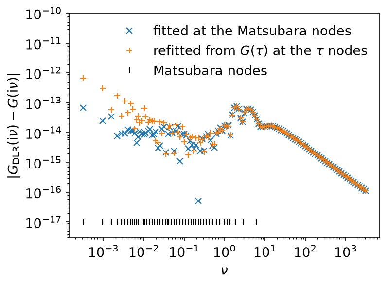
The coefficients themselves are not well determined: the condition numbers of these node matrices are large, and two fits can give different \(c_p\) that produce the same \(G\). Compare values of \(G\), not coefficients.
\(\varepsilon\) decides the number of poles, and asking for too much does
not pay. At \(\varepsilon = 10^{-15}\) the ID returns 192 poles instead of 98, the
node matrices become numerically singular (condition_number returns
infinity), and \(G(\mathrm{i}\nu)\) comes out less accurate, not more.
\(10^{-14}\) is about as small as \(\varepsilon\) usefully goes in double
precision, which is why the examples here pass it explicitly rather than
rely on the default.
A DLR from an IR basis
If your calculation already uses an IR basis, from_ir builds a DLR from it.
The poles are the roots of \(v_L(\omega)\), the first basis function the
truncation discarded, so there are exactly basis.size() of them, one per
basis function, whatever \(\varepsilon\) the basis was built with. This
choice is heuristic, but it makes the matrix \(v_l(\omega_p)\) well
conditioned, so that the IR and DLR coefficients convert into each other
without losing digits.
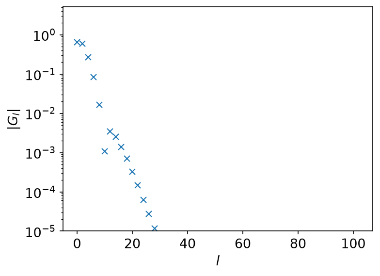
The model is the same semicircle at \(\Lambda = 10^4\), \(\omega_\mathrm{max} = 1\) and \(\varepsilon = 10^{-15}\): a basis of 104 functions, and therefore 104 poles. These are the exact IR coefficients \(g_l\):
    let kernel = LogisticKernel::new(BETA * WMAX)?;
    let basis = FiniteTempBasis::<LogisticKernel, Fermionic>::new(kernel, BETA, Some(EPS), None)?;
    // One pole per basis function, at the roots of the first discarded v_l.
    let dlr = DiscreteLehmannRepresentation::<Fermionic>::from_ir(&basis)?;
    let poles = dlr.poles().to_vec();
    assert_eq!(
        poles.len(),
        basis.size(),
        "an IR-derived DLR has one pole per basis function"
    );
An IR-derived DLR carries the transform to its source basis. from_ir_nd and
to_ir_nd are the two directions. They transform one axis of an array, so a
one-dimensional \(g_l\) goes in as a rank-1 tensor:
    // g_l -> c_p: one axis of a tensor, here a rank-1 tensor.
    let g_l_tensor = TypedTensor::from_vec_col_major(vec![basis.size()], g_l.clone())?;
    let c_p = dlr.from_ir_nd::<f64>(None, &g_l_tensor, 0)?;
    // c_p -> g_l
    let g_l_reconstructed = dlr.to_ir_nd::<f64>(None, &c_p, 0)?;
These two calls exist only on a DLR built by from_ir or
from_ir_with_poles. On a DLR built by new there is no IR basis to convert
to, and they return Error::NotSupported; use the DLR’s own nodes, as above.
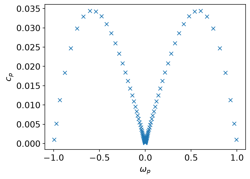
The coefficients sit on the poles like a sampled spectral function, which is what they are:
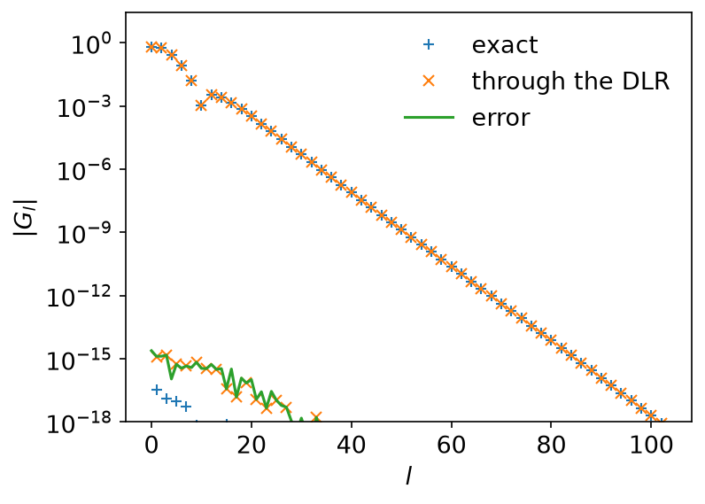
The round trip \(g_l \to c_p \to g_l\) costs nothing but rounding error:
Why bother
Because of what the poles let you do afterwards. The DLR is an analytic function of \(\mathrm{i}\nu\). Evaluating it anywhere is a sum over 104 terms, with no basis functions and no sampling matrix:
    // The DLR needs no basis functions here: it is a sum over poles,
    // G(iν) = Σ_p c_p w_p / (iν − ω_p). The weight w_p is 1 for fermions and
    // tanh(βω_p/2) for bosons.
    let weights = dlr.pole_weights();
    let g_iv_dlr: Vec<Complex64> = nu
        .iter()
        .map(|&nu| {
            (0..poles.len())
                .map(|p| {
                    *c_p.get(&[p]).unwrap() * weights[p] / (Complex64::new(0.0, nu) - poles[p])
                })
                .sum()
        })
        .collect();
For fermions \(w_p = 1\); written with pole_weights(), the same sum is
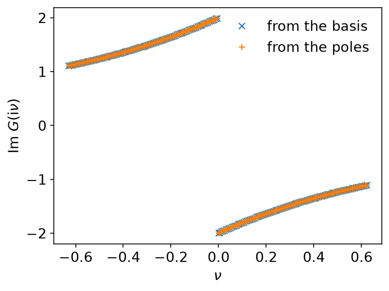
correct for bosons too. The answer agrees with the IR basis to the accuracy of
the basis, here out to \(|n| = 2000\), far beyond the sampling frequencies:
The same sum works for \(\tau\), for real frequencies just above the axis, and for products of Green’s functions, where the pole structure is what makes the convolution cheap.
Key API pieces
| What you want | What to call |
|---|---|
| a DLR without an IR basis (default) | DiscreteLehmannRepresentation::new(beta, wmax, eps), DlrBuilder |
| its sampling points | tau_nodes, matsubara_nodes; or TauSampling::new(&dlr), MatsubaraSampling::new(&dlr) |
| values → \(c_p\), \(c_p\) → values | fit, evaluate of either sampling object; MatsubaraSampling::fit_real, evaluate_real for real \(c_p\) |
| the default poles of an IR basis | DiscreteLehmannRepresentation::from_ir (trait DlrFromIr) |
| poles you chose yourself | DiscreteLehmannRepresentation::from_ir_with_poles |
| where the poles are | poles |
| the weights \(w_p\) | pole_weights |
| \(g_l \to c_p\), \(c_p \to g_l\) (IR-derived DLR only) | from_ir_nd, to_ir_nd |
A DiscreteLehmannRepresentation is itself a Basis, so evaluate_tau and
evaluate_matsubara work on it as they do on the IR basis.
Running it
From docs/tutorial-code:
cargo run --profile ci --bin dlr
uv run --project ../plotting python ../plotting/dlr_plot.py
MiniPole: a few complex poles from Matsubara data
sparse_ir::minipole is a Rust port of
Green-Phys/MiniPole (MIT License),
the reference implementation of the minimal pole method: L. Zhang and E. Gull,
Phys. Rev. B 110, 035154 (2024),
and, for matrix-valued functions, L. Zhang, Y. Yu and E. Gull,
Phys. Rev. B 110, 235131 (2024).
Both rest on the ESPRIT algorithm, available on its own as sparse_ir::esprit.
The Python tutorials have
no MiniPole notebook; this page is written for the Rust library.
MiniPole approximates a Green’s function by a small number of poles that are allowed to leave the real axis,
\[ G(z) \simeq C + \sum_{j} \frac{A_j}{z-\xi_j}. \]
The DLR uses a fixed grid of real poles \(\omega_p\) that works for every function with the same \(\beta\) and \(\omega_{\max}\). MiniPole instead adapts the poles \(\xi_j\) to one particular function. The result is much smaller than a DLR, it evaluates anywhere in the complex plane, and \(-\mathrm{Im}\,G(\omega+\mathrm{i}0)/\pi\) gives a spectral function, so it doubles as a tool for analytic continuation. A continuous spectrum is represented by poles pushed below the real axis.
What MiniPole gives you
Take the semicircular density of states \(\rho(\omega) = (2/\pi)\sqrt{1-\omega^2}\) on \([-1, 1]\). Its Green’s function \(G(z) = \int \mathrm{d}\omega\,\rho(\omega)/(z-\omega)\) is \(G(z) = 2\left(z - \sqrt{z-1}\sqrt{z+1}\right)\) on the physical sheet. With \(\beta=100\) and \(\omega_{\max}=1.5\), build a DLR, fit its coefficients to the exact \(G(\mathrm{i}\nu_n)\) at the DLR’s own sparse Matsubara nodes, and compress the coefficients with MiniPole:
use num_complex::Complex64;
use sparse_ir::minipole::{MiniPoleDlrParams, MiniPoleResult, mini_pole_dlr_from};
use sparse_ir::{
    Bosonic, DiscreteLehmannRepresentation, Fermionic, MatsubaraSampling, TypedTensor,
};
use std::error::Error;
use std::f64::consts::PI;
/// Semicircular DOS rho(w) = (2/pi) sqrt(1 - w^2) on [-1, 1]. Its Green's
/// function on the physical sheet is G(z) = 2 (z - sqrt(z-1) sqrt(z+1)).
fn semicircle(z: Complex64) -> Complex64 {
    2.0 * (z - (z - 1.0).sqrt() * (z + 1.0).sqrt())
}

/// Largest |G_MP(iv_n) - G(iv_n)| over the fermionic frequencies
/// iv_n = i n pi / beta with odd n, 0 < n < 2000. The poles lie in the lower
/// half plane, so G_MP represents G in the upper half plane only.
fn max_matsubara_error(rep: &MiniPoleResult, beta: f64) -> Result<f64, Box<dyn Error>> {
    let z: Vec<Complex64> = (0..1000)
        .map(|m| Complex64::new(0.0, (2 * m + 1) as f64 * PI / beta))
        .collect();
    let got = rep.evaluate(&z)?;
    Ok(got
        .host_data()?
        .iter()
        .zip(&z)
        .map(|(g, &zi)| (*g - semicircle(zi)).norm())
        .fold(0.0, f64::max))
}
    let (beta, wmax) = (100.0, 1.5);
    // An IR-independent DLR and its sparse Matsubara nodes.
    let dlr = DiscreteLehmannRepresentation::<Fermionic>::new(beta, wmax, 1e-12)?;
    let sampling = MatsubaraSampling::new(&dlr)?;
    let values: Vec<Complex64> = sampling
        .sampling_points()
        .iter()
        .map(|n| semicircle(n.value_imaginary(beta)))
        .collect();
    let values = TypedTensor::from_vec_col_major(vec![values.len()], values)?;
    let coeffs = sampling.fit_nd(None, &values, 0)?;

    // Contour from iw_5 = 11 pi / beta up to the default nmax = beta;
    // ESPRIT tolerance err = 1e-8.
    let rep = mini_pole_dlr_from(&dlr, &coeffs, &MiniPoleDlrParams::new(5, 1e-8))?;
    for pole in &rep.pole_location {
        println!("pole {:+.4} {:+.4}i", pole.re, pole.im);
        assert!(pole.im < 0.0, "pole {pole} is not in the lower half plane");
    }
    let error = max_matsubara_error(&rep, beta)?;
    println!(
        "{} poles (DLR size {}), max |G_MP - G| on iv_n = {error:.1e}",
        rep.pole_location.len(),
        dlr.poles().len()
    );
    assert!(error < 1e-3, "Matsubara error {error}");
Ok::<(), Box<dyn std::error::Error>>(())
The DLR has 39 poles. MiniPole returns five: \(\pm 0.940 - 0.151\mathrm{i}\), \(\pm 0.643 - 0.516\mathrm{i}\) and \(-0.737\mathrm{i}\). The code asserts that every pole lies in the lower half plane and that \(|G_{\rm MP}(\mathrm{i}\nu_n) - G(\mathrm{i}\nu_n)| < 10^{-3}\) for the positive fermionic frequencies \(\nu_n = n\pi/\beta\), \(n\) odd, \(n < 2000\); the actual maximum is \(1.8\times 10^{-4}\).
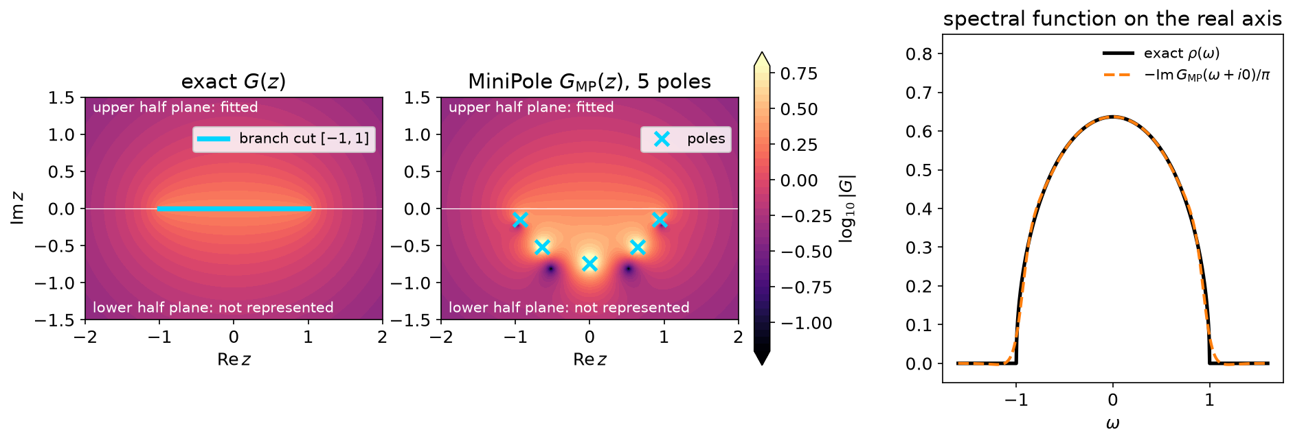
Left: \(\log_{10}|G(z)|\) of the exact function, analytic everywhere except on the branch cut \([-1,1]\). Middle: the MiniPole reconstruction. In the upper half plane, where the Matsubara data live, the two panels agree. The branch cut is replaced by five poles in the lower half plane; there, \(G_{\rm MP}\) is not meant to reproduce \(G\). Right: the spectral function \(-\mathrm{Im}\,G_{\rm MP}(\omega+\mathrm{i}0)/\pi\) against the exact semicircle. Since no pole is on or above the real axis, \(G_{\rm MP}(\omega+\mathrm{i}0)\) is simply \(G_{\rm MP}(\omega)\).
The number of poles is controlled by the ESPRIT tolerance err
(\(\varepsilon\) in the conventions).
It grows slowly as err decreases:
    // Fewer poles for a looser tolerance; err is not an error bound.
    let mut errs = Vec::new();
    let mut counts = Vec::new();
    let mut errors = Vec::new();
    for err in [1e-4, 1e-6, 1e-8, 1e-10] {
        let rep = mini_pole_dlr_from(&dlr, &coeffs, &MiniPoleDlrParams::new(5, err))?;
        assert!(rep.pole_location.iter().all(|p| p.im < 0.0));
        let error = max_matsubara_error(&rep, beta)?;
        println!(
            "err = {err:.0e}: {} poles, max error {error:.1e}",
            rep.pole_location.len()
        );
        errs.push(err);
        counts.push(rep.pole_location.len() as f64);
        errors.push(error);
    }
err | poles | max \(\lvert G_{\rm MP}-G\rvert\) on \(\mathrm{i}\nu_n\) |
|---|---|---|
| \(10^{-4}\) | 3 | \(7.4\times 10^{-3}\) |
| \(10^{-6}\) | 4 | \(1.2\times 10^{-3}\) |
| \(10^{-8}\) | 5 | \(1.8\times 10^{-4}\) |
| \(10^{-10}\) | 6 | \(3.0\times 10^{-5}\) |
err is a tolerance for the singular values inside ESPRIT. It is not a
bound on the error of \(G\): with err = 1e-8 the Matsubara error is
\(1.8\times 10^{-4}\).
Three entry points
| Function | Input | Frequencies | n0 means | Upper end of the contour |
|---|---|---|---|---|
mini_pole_dlr_from(&dlr, &coeffs, &p) | DLR coefficients \(g_l\) from MatsubaraSampling::fit_nd | contour \(\omega_n = (2n+1)\pi/\beta\), also for bosons | contour index | nmax (default \(\beta\)) |
mini_pole_dlr(&residues, &locations, beta, &p) | real poles and their actual residues | same as above | contour index | nmax |
mini_pole(&values, &freqs, &p) | \(G\) on a uniform, non-negative grid of physical frequencies \(\omega_n\) (real numbers, not indices) | as supplied | position in the array (N0::Auto by default) | last element |
C API spir_minipole_from_matsubara | as mini_pole | reduced indices \(n\), converted as \(\omega = n\pi/\beta\) | position in the array (\(<0\): automatic) | last element |
p is MiniPoleDlrParams for the first two and MiniPoleParams for
mini_pole. mini_pole_dlr_from forms the residues \(A_l = g_l w_l\) with
dlr.pole_weights() itself; bosonic DLR coefficients are not residues, so do
not pass them to mini_pole_dlr. The contour index of the DLR entry points is
not the reduced Matsubara index \(n\) used elsewhere in the library
(\(\mathrm{i}\nu_n = \mathrm{i}n\pi/\beta\)). The C function
spir_minipole_from_dlr follows mini_pole_dlr_from.
All of them return a MiniPoleResult with pole_location (\(\xi_j\), sorted
by real part), pole_weight (\(A_j\)), constant (\(C\)), and
evaluate(&z) for arbitrary complex \(z\). The full list of parameters
(symmetry, fixed pole count, N0::Auto, constant term, residue plane, C
arguments) is in the
sparse_ir::minipole module documentation.
Choosing the contour and err
MiniPole does not work on the Matsubara values directly. It maps the complex plane, cut along a segment of the imaginary axis, conformally onto the unit disk, so that the segment becomes the unit circle. It then computes moments of \(G\) along the segment and runs ESPRIT on those moments. For the DLR entry points the segment is
\[ [\mathrm{i}\omega_{n_0},\ \mathrm{i}\omega_{n_{\max}}],\qquad \omega_n=(2n+1)\pi/\beta . \]
n0sets the lower end. There is no automatic choice for DLR input.nmaxsets the upper end;Nonemeans \(n_{\max}=\beta\) (the number, in the units of the input). It is a floating-point cutoff, not a number of samples, and must exceedn0.erris the ESPRIT tolerance described above: set it at or above the noise level of the data.
The contour matters. Keep the same DLR coefficients and err = 1e-8, and
start the contour at three different points:
    // Same coefficients and err, three lower ends of the contour.
    let mut scan = Vec::new();
    for n0 in [0, 2, 5] {
        let rep = mini_pole_dlr_from(&dlr, &coeffs, &MiniPoleDlrParams::new(n0, 1e-8))?;
        let upper = rep.pole_location.iter().filter(|p| p.im > 0.0).count();
        let error = max_matsubara_error(&rep, beta)?;
        println!(
            "n0 = {n0}: {} poles, {upper} in the upper half plane, max error {error:.1e}",
            rep.pole_location.len()
        );
        scan.push((n0, upper, error, rep));
    }
    // n0 = 0 and 2 give spurious upper-half-plane poles; n0 = 5 does not.
    assert!(
        scan.iter()
            .all(|(n0, upper, ..)| (*n0 == 5) == (*upper == 0))
    );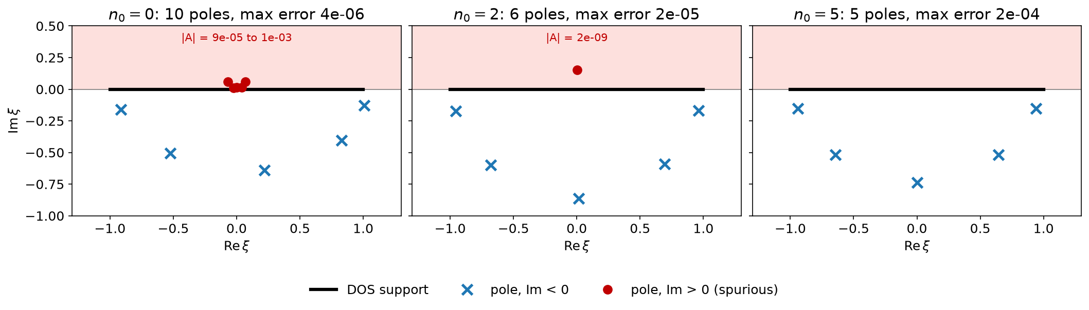
For n0 = 0 and n0 = 2 MiniPole returns extra poles in the upper half
plane, near the origin. Their weights are tiny (\(10^{-4}\) to
\(10^{-3}\) and \(2\times 10^{-9}\)), and the Matsubara error is in fact
smaller than for n0 = 5 (\(4\times10^{-6}\) and \(2\times10^{-5}\)
against \(2\times10^{-4}\)). But a pole with \(\mathrm{Im}\,\xi>0\) makes
\(G_{\rm MP}\) non-analytic in the upper half plane, so it cannot be a
retarded Green’s function. With n0 = 5 all poles are in the lower half plane.
The lesson: a small residual on the Matsubara axis does not validate the
contour; a pole in the upper half plane is the sign of a bad contour.
A harder case: a low-energy bosonic pair
Now take a bosonic susceptibility with \(\beta=20\), \(\omega_{\max}=3\), and the odd spectral function
\[ \rho(\omega)=\sum_j A_j\delta(\omega-\xi_j),\qquad (\xi_j,A_j)=(-1.2,-0.2),(-0.1,-0.3),(0.1,0.3),(1.2,0.2). \]
Thus \(\rho(-\omega)=-\rho(\omega)\), the inner pair has \(\beta|\xi|=2\), and \(\chi(0)=-19/3\) is finite. Fit the exact \(\chi(z)=\sum_j A_j/(z-\xi_j)\) at the DLR’s sparse Matsubara nodes and compress the coefficients. The DLR contour uses \((2n+1)\pi/\beta\) here too, even though the data are bosonic:
use num_complex::Complex64;
use sparse_ir::minipole::{MiniPoleDlrParams, MiniPoleResult, mini_pole_dlr_from};
use sparse_ir::{
Bosonic, DiscreteLehmannRepresentation, Fermionic, MatsubaraSampling, TypedTensor,
};
use std::error::Error;
use std::f64::consts::PI;
let (beta, wmax) = (20.0, 3.0);
// Odd spectral function: residues have opposite signs at +/- xi.
let spectrum = [(-1.2, -0.2), (-0.1, -0.3), (0.1, 0.3), (1.2, 0.2)];
let exact = |z: Complex64| -> Complex64 { spectrum.iter().map(|&(xi, a)| a / (z - xi)).sum() };
let dlr = DiscreteLehmannRepresentation::<Bosonic>::new(beta, wmax, 1e-12)?;
let sampling = MatsubaraSampling::new(&dlr)?;
let values: Vec<Complex64> = sampling
.sampling_points()
.iter()
.map(|n| exact(n.value_imaginary(beta)))
.collect();
let values = TypedTensor::from_vec_col_major(vec![values.len()], values)?;
let coeffs = sampling.fit_nd(None, &values, 0)?;
// These contour parameters resolve this particular low-energy pair.
let params = MiniPoleDlrParams {
nmax: Some(50.0),
..MiniPoleDlrParams::new(5, 1e-8)
};
let poles = mini_pole_dlr_from(&dlr, &coeffs, ¶ms)?;
assert_eq!(poles.pole_location.len(), 4);
// Independent analytic checks: pole and residue errors below 1e-3, and
// the static value chi(0) within 1 %.
for ((location, weight), &(xi, a)) in poles
.pole_location
.iter()
.zip(poles.pole_weight.host_data()?)
.zip(&spectrum)
{
assert!((*location - xi).norm() < 1e-3, "pole {xi}: {location}");
assert!((*weight - a).norm() < 1e-3, "residue {a}: {weight}");
}
let zero = Complex64::new(0.0, 0.0);
let chi0 = poles.evaluate(&[zero])?.host_data()?[0];
assert!((chi0 - exact(zero)).norm() < 1e-2 * exact(zero).norm());
Ok::<(), Box<dyn std::error::Error>>(())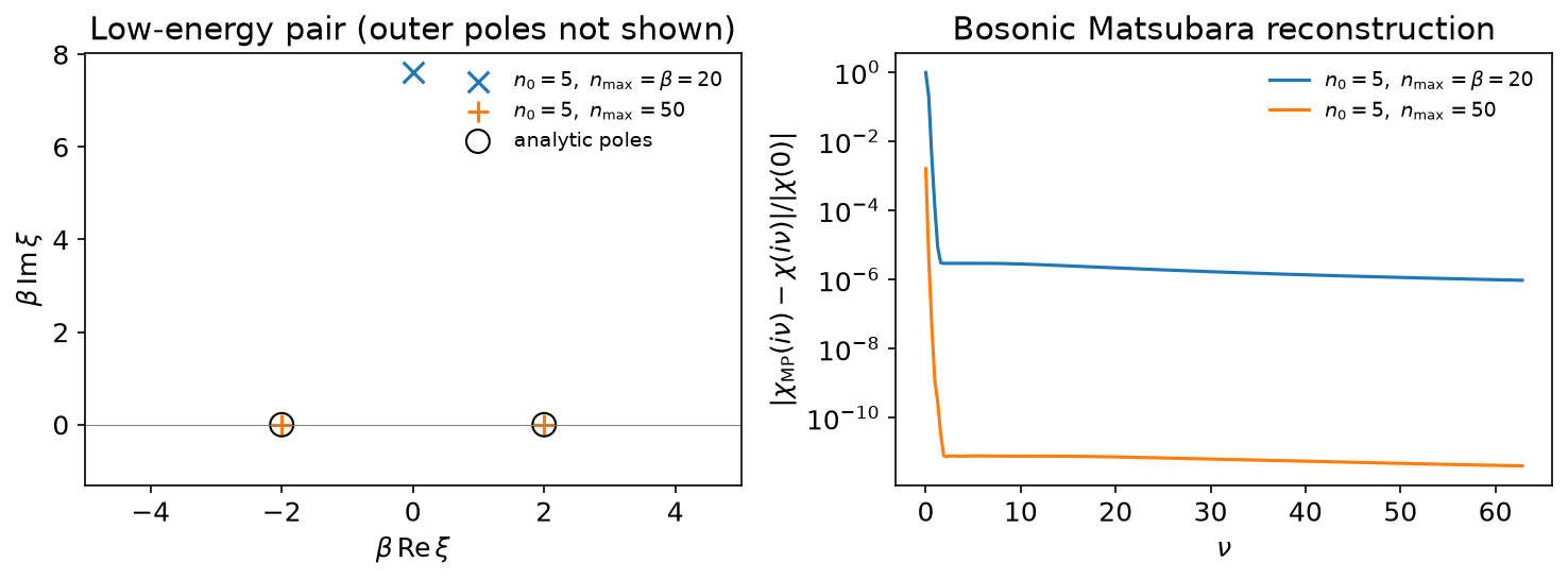
With n0 = 5, err = 1e-8 and the default nmax = beta = 20, MiniPole
returns three poles: the low-energy pair is merged into a single pole near
\(0.380\mathrm{i}\), again in the upper half plane. Extending the contour to
nmax = 50 gives four poles that match the exact ones to \(10^{-3}\), and
\(\chi_{\rm MP}(0)\) within 1 %. The left panel shows the inner poles (the
outer pair at \(\pm1.2\) is not shown); the right panel shows the error at
the bosonic frequencies \(\nu_m = 2m\pi/\beta\), including \(m=0\),
normalized by \(|\chi(0)|\).
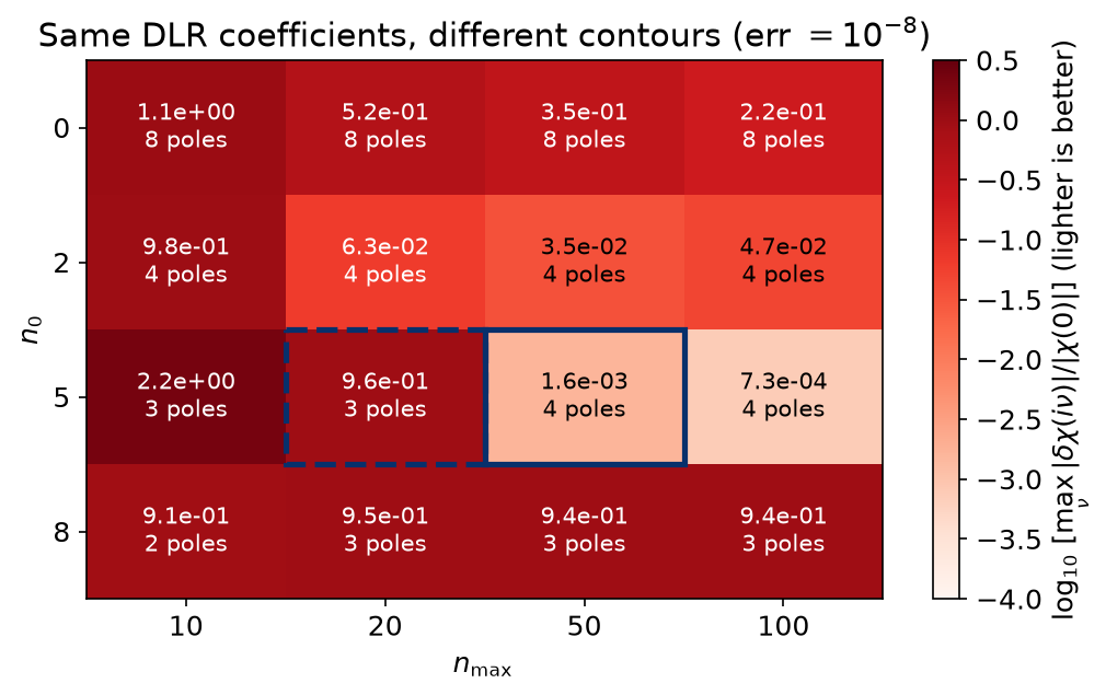
Each cell uses the same DLR coefficients and err = 1e-8. The number is
\(\max_{0\le m\le200}|\chi_{\rm MP}(\mathrm{i}\nu_m)-\chi(\mathrm{i}\nu_m)|/|\chi(0)|\)
and the second line the pole count; lighter cells are better. The dashed box
is the default contour, the solid box the one used above. Only n0 = 5 with
nmax = 50 or 100 brings the error below \(10^{-2}\). A longer contour is not a universal
cure, and neither n0 = 5 nor nmax = 50 is a general recommendation.
Practical checklist
- Compare a few contours (
n0,nmax) on the same data rather than trusting one. - Reject any result with a pole in the upper half plane.
- Check that the poles and residues are stable when the contour or
errchanges slightly. - Check the reconstruction at frequencies not used in the fit, especially near zero frequency.
- With noisy data, set
errat or above the noise level instead of asking for ever more poles.
A good fit at high Matsubara frequencies does not prove that a low-energy feature or the static response is right, and fitting imaginary frequencies does not guarantee a unique real-axis continuation for noisy data. The examples here have an exact answer to compare with; for measured data, stability and held-out residuals are diagnostics, not proof that the poles are physical.
Reproduce the figures
From docs/tutorial-code:
cargo run --profile ci --bin minipole
uv run --project ../plotting python ../plotting/minipole_plot.py
The binary writes CSV tables under docs/tutorial-code/data/minipole/; the
plotting script only reads them.
Analytic continuation
Ported from the Python notebook
analytic_continuation_py.ipynb
of sparse-ir-tutorial.
The program that produced every number and figure on this page is
docs/tutorial-code/src/bin/analytic_continuation.rs; the code below is
included from it.
Going from a spectral function to a Green’s function is a smoothing integral and always works. This page looks at the inverse, from \(G\) back to \(\rho(\omega)\), and shows why it is ill posed: what fails, what two simple regularisers buy, and why the IR coefficients of \(\rho\) are the wrong unknowns. Sparse modeling then solves one such problem in full, and MiniPole takes a different route by fitting poles.
The problem
\[ G(\tau) = -\int \mathrm{d}\omega, K(\tau, \omega), \rho(\omega) \]
In the basis this reads \(G_l = -s_l \rho_l\), one number at a time, and it inverts in one line:
\[ \rho(\omega) = -\sum_l \frac{G_l}{s_l} v_l(\omega). \]
Every \(s_l\) is strictly positive, so the inverse exists. It is also useless, because the \(s_l\) fall off exponentially:
use sparse_ir::Matrix;
use sparse_ir::{Basis, Fermionic, FiniteTempBasis, LogisticKernel};
// These must agree with `scripts/make_analytic_continuation_input.py`.
const BETA: f64 = 40.0;
const WMAX: f64 = 2.0;
const EPS: f64 = 2e-8;
    let kernel = LogisticKernel::new(BETA * WMAX)?;
    let basis = FiniteTempBasis::<LogisticKernel, Fermionic>::new(kernel, BETA, Some(EPS), None)?;
    let size = basis.size();
    let s = basis.s().to_vec();
Ok::<(), Box<dyn std::error::Error>>(())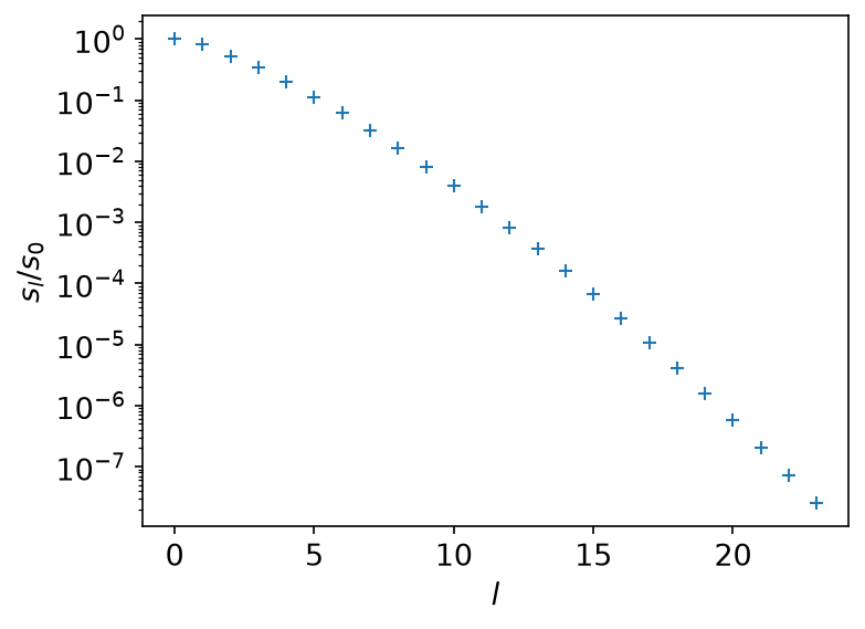
At \(\beta = 40\), \(\omega_\mathrm{max} = 2\) and \(\varepsilon = 2 \times 10^{-8}\) the basis has 24 functions and \(s_{23}/s_0 \approx 2.5 \times 10^{-8}\). Dividing by that last singular value multiplies whatever error rides on \(G_{23}\) by forty million. There is no algorithm that avoids this: the information about the fine structure of \(\rho\) is not in \(G\) to be recovered. All a method can do is choose what to put in its place.
Two models
Both are sums of normalised semicircles, so their exact \(\rho_l\) can be computed to machine precision and used as ground truth. One fills the band; the other is the same band split by a gap.
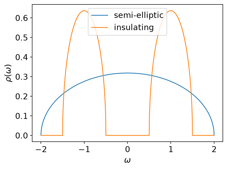
shifted_semicircle_overlaps (a tutorial helper) computes \(\rho_l\) of one
semicircle by quadrature, and \(G_l = -s_l \rho_l\):
    let rho_semi = shifted_semicircle_overlaps(&basis, 0.0, WMAX, 1.0);
    let rho_insul = {
        let right = shifted_semicircle_overlaps(&basis, WMAX / 2.0, WMAX / 4.0, 0.5);
        let left = shifted_semicircle_overlaps(&basis, -WMAX / 2.0, WMAX / 4.0, 0.5);
        right
            .iter()
            .zip(&left)
            .map(|(a, b)| a + b)
            .collect::<Vec<_>>()
    };
    let g_semi = coefficients(&s, &rho_semi);
    let g_insul = coefficients(&s, &rho_insul);
/// `Gₗ = −sₗ ρₗ`.
fn coefficients(s: &[f64], rho_l: &[f64]) -> Vec<f64> {
    s.iter().zip(rho_l).map(|(sl, rho)| -sl * rho).collect()
}
Then noise is added to \(G_l\), at \(0.3,(s_{L-1}/s_0)\) of \(\lVert G \rVert\) — deliberately of the same size as the smallest coefficient the basis still resolves.
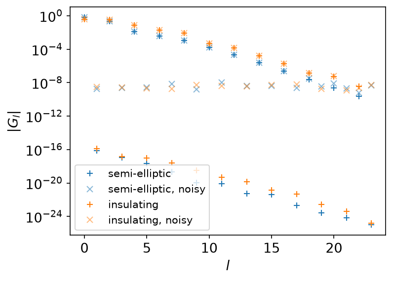
The noise is far below every coefficient that matters and level with the ones
at the end. The standard-normal draws are read from
docs/tutorial-code/input/analytic_continuation/noise.csv.
Truncated SVD
The first regulariser is the blunt one: keep \(\rho_l = -G_l/s_l\) for \(l < L’\) and throw the rest away.
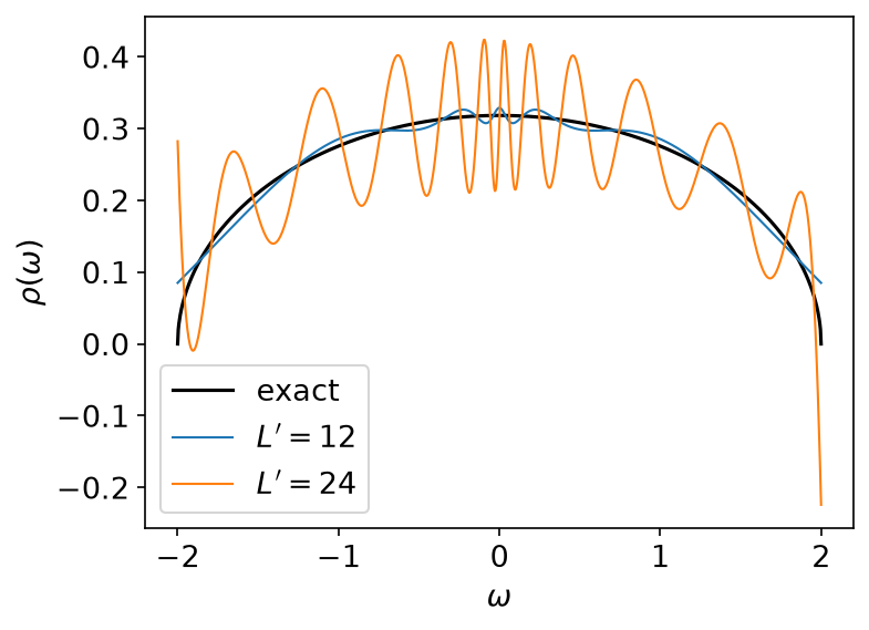
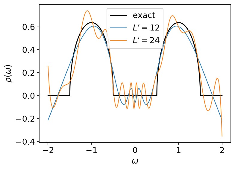
\(L’ = 12\) gets the shape right. \(L’ = 24\) — using everything the basis has — turns the answer into ringing of amplitude 0.2 around a function whose peak is 0.32. Using more of the data made the answer worse, which is the whole difficulty in one picture.
The insulating model says the same thing with a sharper edge:
Ridge regression
The second regulariser is smooth: minimise \(\lVert G - (-s\rho) \rVert^2 + \alpha^2 \lVert \rho \rVert^2\). Because the problem is diagonal in the basis, the solution is diagonal too,
\[ \rho_l = -\frac{s_l}{s_l^2 + \alpha^2}, G_l, \]
which passes the large singular values through unchanged and rolls the small ones off instead of dividing by them.
    let ridge: Vec<f64> = s.iter().map(|sl| -sl / (sl * sl + alpha * alpha)).collect();
    let rho_l_semi_ridge: Vec<f64> = ridge
        .iter()
        .zip(&g_semi_noisy)
        .map(|(r, g)| r * g)
        .collect();
    let rho_l_insul_ridge: Vec<f64> = ridge
        .iter()
        .zip(&g_insul_noisy)
        .map(|(r, g)| r * g)
        .collect();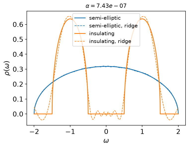
With \(\alpha = 100 \times \text{noise}\) both models come back recognisably. Note what is left over: the reconstruction goes negative inside the gap. A density of states cannot do that, and no amount of tuning \(\alpha\) will stop it, because nothing in the method knows that \(\rho \geq 0\).
Why ρl is the wrong unknown
It is tempting to conclude that the fix is a better penalty on \(\rho_l\). It is not, and the reason is worth stating plainly: \(G_l\) is compact, \(\rho_l\) is not. The basis is small because \(s_l\) makes it small — and \(s_l\) belongs to \(G\), not to \(\rho\).
Take four delta peaks, \(\rho(\omega) = \sum_i \delta(\omega - \omega_i)\), so that \(\rho_l = \sum_i v_l(\omega_i)\):
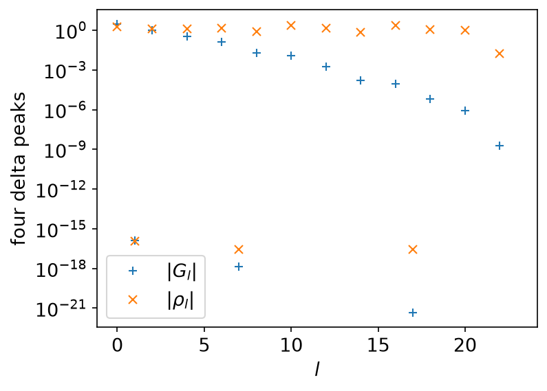
\(G_l\) falls off the way it always does. \(\rho_l\) does not fall off at all — it is still of order one at \(l = 23\), and would be at \(l = 200\). Truncating it at \(L’\) is not an approximation of anything; a penalty on \(\sum_l |\rho_l|^2\) is a penalty on coefficients that were never going to become small.
A spectrum made of a few poles is, on the other hand, exactly the case that pole-fitting methods handle well. MiniPole uses ESPRIT to fit a small number of poles and residues directly to Matsubara data, instead of expanding \(\rho\) in any basis.
A real-axis basis instead
So expand \(\rho\) on the real axis rather than in the IR basis:
\[ \rho(\omega) = \sum_{m} a_m, f(\omega - \omega_m), \qquad f(\omega) = \frac{1}{\pi}\frac{\eta}{\omega^2 + \eta^2}. \]
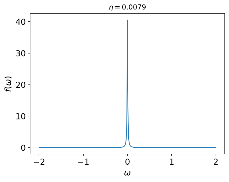
\(f\) is a probability density, so \(a_m \geq 0\) gives \(\rho \geq 0\) and \(\sum_m a_m = 1\) gives the sum rule — both of them constraints a solver can impose exactly, neither of them expressible in the IR coefficients. The width \(\eta\) is what is left to choose; \(\eta = 0.1,\pi/\beta\) is narrow enough to resolve structure on the scale of the temperature and wide enough not to be a set of delta functions.
The data then enter through
\[ G_l = \sum_m K_{lm} a_m, \qquad K_{lm} = -s_l \int \mathrm{d}\omega, v_l(\omega) f(\omega - \omega_m), \]
which is an ordinary constrained least-squares problem in \(a\).
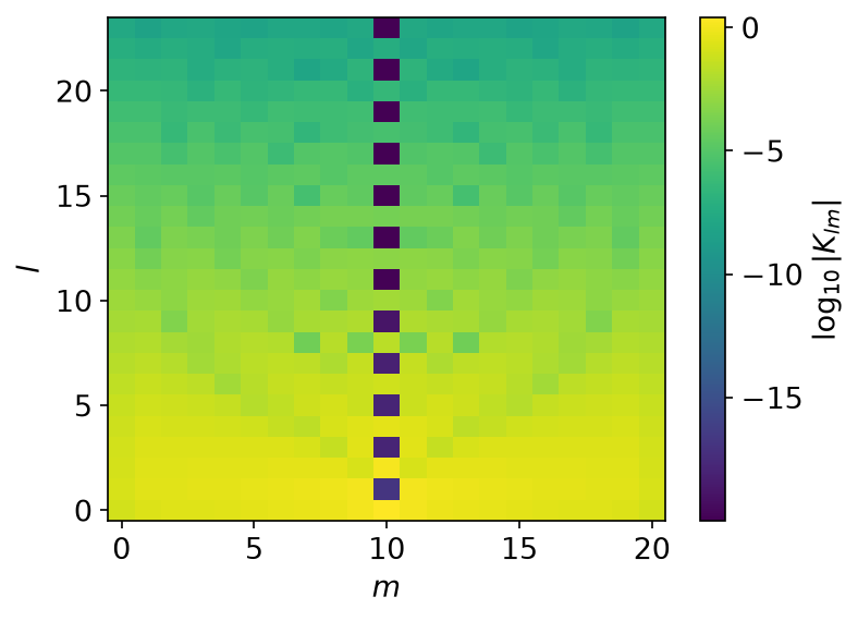
Computing \(K_{lm}\) is the one place this example does real numerical work. \(\eta\) is about a hundredth of the spacing between the basis’ knots, so quadrature on the knots steps straight over the peak of \(f\). The substitution \(\omega = \omega_m + \eta \tan t\) turns \(f(\omega - \omega_m),\mathrm{d}\omega\) into \(\mathrm{d}t/\pi\) and spreads the peak across the whole interval, leaving a polynomial to integrate:
/// `∫ dω vₗ(ω) f(ω − centre)` over the basis' ω range, to machine precision.
///
/// `η` is a small fraction of the knot spacing, so quadrature on the knots
/// alone would step straight over the peak. The substitution
/// `ω = centre + η tan t` turns `f(ω − centre) dω` into `dt/π` and spreads the
/// peak over the whole integration range; the knots come along as the segment
/// edges in `t`, where `vₗ` is still a polynomial in `ω`.
fn lorentz_overlaps(
    basis: &FiniteTempBasis<LogisticKernel, Fermionic>,
    centre: f64,
    eta: f64,
) -> Vec<f64> {
    let v = basis.v();
    let edges: Vec<f64> = v
        .get_knots(None)
        .into_iter()
        .map(|omega| ((omega - centre) / eta).atan())
        .collect();
    // tan t varies fast at the ends of each segment, so take more points than
    // the polynomial degree alone would need.
    let order = v.get_polyorder() + 24;

    (0..basis.size())
        .map(|l| {
            let poly = &v[l];
            integrate_segments(
                |t| poly.evaluate(centre + eta * t.tan()) / std::f64::consts::PI,
                &edges,
                order,
            )
        })
        .collect()
}
What this page stops short of
This page does not solve the constrained least-squares problem in \(a\). Sparse modeling solves a related one: an L1-regularised fit in the IR coefficients \(\rho_l\), without \(\rho \geq 0\) or the sum rule. Solving on the Lorentzian basis with both constraints imposed is the subject of the maximum-entropy and sparse-modeling literature, and is past where a tutorial ends.
Running it
From docs/tutorial-code:
$ cargo run --release --bin analytic_continuation
The program writes CSV tables to docs/tutorial-code/data/analytic_continuation/.
The figures are drawn from those tables; from the repository root, run
uv run --project docs/plotting python docs/plotting/analytic_continuation_plot.py.
The noise is committed rather than drawn at run time, so that this program and
its Python counterpart,
docs/tutorial-code/scripts/reference_analytic_continuation.py, use the same
numbers; the header of noise.csv says where the draws came from.
Key API pieces
From sparse-ir:
| What you want | What to call |
|---|---|
| the singular values | FiniteTempBasis::s |
| \(v_l\) on a grid of ω | Basis::evaluate_omega |
| the knots the basis is piecewise-polynomial on | basis.v().get_knots(None) |
| one \(v_l\) as a polynomial | basis.v()[l].evaluate(omega) |
| the degree to integrate exactly | basis.v().get_polyorder() |
From the tutorial crate (sparse_ir_tutorial, not part of the library):
| What you want | What to call |
|---|---|
| \(\rho_l\) of a semicircle | shifted_semicircle_overlaps |
| composite Gauss–Legendre quadrature over segments | integrate_segments |
Sparse modeling
Ported from the Python notebook
spm_py.ipynb
of sparse-ir-tutorial.
The program that produced every number and figure on this page is
docs/tutorial-code/src/bin/spm.rs; the code below is included from it.
This page solves one analytic-continuation problem end to end: from a noisy \(G(\tau)\) back to the \(\rho(\omega)\) that produced it, with an L1 penalty on the IR coefficients. The problem is ill posed: the kernel smooths, so the inverse sharpens, and it sharpens the noise along with the signal. Analytic continuation looks at that difficulty itself and at two simpler regularisers.
The IR basis makes the difficulty explicit rather than making it go away. In the basis,
\[ G_l = -s_l \rho_l, \]
so recovering \(\rho_l\) means dividing by \(s_l\). The singular values fall off exponentially, so past the point where \(s_l\) drops below the noise level, the data say nothing at all about \(\rho_l\). Sparse modeling is the choice to set those coefficients to zero rather than to let them be whatever the noise dictates.
The problem
Minimise, over the IR coefficients \(x_l = \rho_l\),
\[ \tfrac12 \lVert y - A x \rVert^2 + \lambda \lVert x \rVert_1, \qquad y_i = -G(\tau_i), \quad A_{il} = u_l(\tau_i), s_l . \]
The first term says the answer must explain the data. The L1 penalty is what makes the solution sparse: unlike a least-squares penalty, it drives coefficients to exactly zero instead of merely making them small. \(\lambda\) decides how many survive.
The data
The notebook downloads a sample Gtau.in from the SpM repository. This port
ships its input instead, docs/tutorial-code/input/spm/gtau.csv. It is
\(G(\tau)\) of the three-Gaussian spectral function from
the transformation page, at \(\beta = 100\) and
\(\omega_\mathrm{max} = 4\), on 401 uniform times \(\tau_i \in [0, \beta]\),
plus independent Gaussian noise of size \(10^{-3}\). Unlike the downloaded
file, it comes with the exact answer.
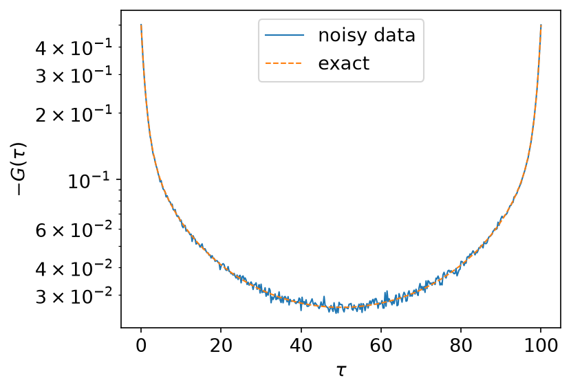
The noise is invisible here — \(10^{-3}\) against a curve of order 1 — and it is what decides how much of the spectrum can be recovered.
    let input = read_table(&input_path(EXAMPLE, "gtau"))?;
    let taus = input.expect_column("tau").to_vec();
    let g_tau = input.expect_column("g_tau").to_vec();
    let g_tau_clean = input.expect_column("g_tau_clean").to_vec();
    let n_tau = taus.len();
Building A
The basis has \(\varepsilon = 10^{-10}\) and 43 functions:
use sparse_ir::Matrix;
use sparse_ir::{Basis, Fermionic, FiniteTempBasis, LogisticKernel};
// These must agree with `scripts/make_spm_input.py`, which wrote the input.
const BETA: f64 = 100.0;
const WMAX: f64 = 4.0;
const EPS: f64 = 1e-10;
    let kernel = LogisticKernel::new(BETA * WMAX)?;
    let basis = FiniteTempBasis::<LogisticKernel, Fermionic>::new(kernel, BETA, Some(EPS), None)?;
    let size = basis.size();
Ok::<(), Box<dyn std::error::Error>>(())
\(A\) is the matrix of basis functions at the sampled times, scaled by the
singular values. evaluate_tau returns \(u_l(\tau_i)\) with the points along
the first axis:
    // `A_{il} = u_l(τ_i) s_l` maps IR coefficients of ρ to −G(τ).
    let u_at_taus: Matrix<f64> = basis.evaluate_tau(&taus)?;
    let mut a = vec![0.0; n_tau * size];
    for i in 0..n_tau {
        for l in 0..size {
            a[i * size + l] = *u_at_taus.get(&[i, l]).unwrap() * basis.s()[l];
        }
    }
    let y: Vec<f64> = g_tau.iter().map(|g| -g).collect();
43 unknowns against 401 equations — and still ill posed, because the last columns of \(A\) are multiplied by singular values of order \(10^{-10}\).
Solving it
sparse_ir_tutorial::fista is the standard proximal-gradient method: a
gradient step on the smooth part, then the proximal operator of the penalty,
with Nesterov momentum in between. For an L1 penalty the proximal operator is
soft thresholding — shrink every coefficient towards zero by a fixed amount and
clip the ones that would cross.
/// Minimises `½‖y − A x‖² + λ‖x‖₁` from `x = 0`.
fn solve(
    a: &[f64],
    y: &[f64],
    rows: usize,
    cols: usize,
    lipschitz: f64,
    lambda: f64,
) -> (Vec<f64>, sparse_ir_tutorial::FistaReport) {
    let mut x = vec![0.0; cols];
    let mut residual = vec![0.0; rows];
    let report = fista(
        &mut x,
        lipschitz,
        |x, grad| {
            multiply(a, cols, x, &mut residual);
            for (r, yi) in residual.iter_mut().zip(y) {
                *r -= yi;
            }
            multiply_transposed(a, rows, cols, &residual, grad);
        },
        |x, step| soft_threshold(x, step * lambda),
        FISTA_MAX_ITER,
        FISTA_TOL,
    );
    (x, report)
}
The step length is \(1/L\), with \(L\) the largest eigenvalue of \(A^\mathsf{T} A\), computed by power iteration. The iteration runs for a fixed budget of 20 000 steps rather than stopping on a tolerance: FISTA’s momentum makes the step-to-step change oscillate rather than fall monotonically, so a small tolerance is either never reached or reached at an unpredictable step. The program checks that every solution has settled to a relative change below \(10^{-6}\) by the end of the budget.
What comes out
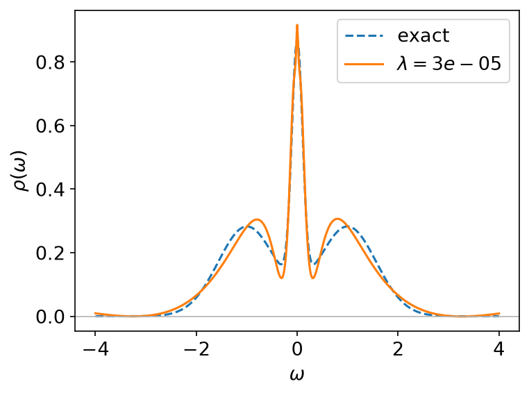
All three peaks come back, the narrow central one included, from data whose noise is a thousand times smaller than the signal but ten million times larger than the smallest singular value that matters.
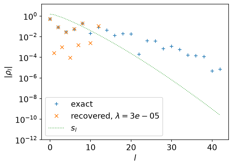
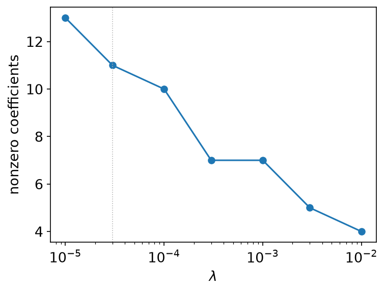
This is the mechanism, in one picture. Only 11 of the 43 coefficients are nonzero; the rest are exactly zero, not small. The cut-off sits where \(s_l\) falls to about \(10^{-3}\) — the noise level. Below that the data carry no information about \(\rho_l\), and the L1 penalty declines to invent any.
Choosing λ
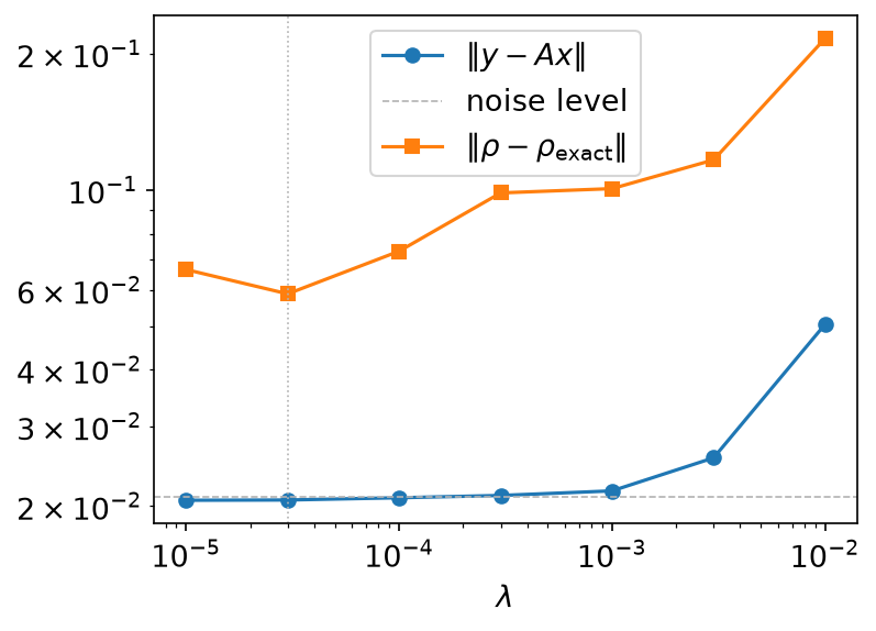
The residual sits flat at the noise level, \(\lVert \delta G \rVert \approx 10^{-3}\sqrt{401} \approx 0.021\), until \(\lambda \approx 10^{-3}\), and then rises: past that point the penalty is discarding signal, not noise. The error against the exact spectrum bottoms out earlier, at \(\lambda = 3\times10^{-5}\), which is the value this page reports.
The two do not coincide, and that is the honest situation: the error curve needs the answer you are trying to find. In practice you have only the residual curve and the noise level, which together bracket \(\lambda\) to about a decade — and within that decade the spectrum barely changes.
What this port leaves out
The notebook solves a constrained version of the same problem: it adds
\(\rho(\omega) \ge 0\) and the sum rule \(\int\mathrm{d}\omega,\rho = 1\)
as hard constraints. Neither has a cheap proximal operator — \(\rho \ge 0\)
is a constraint on \(V x\), not on \(x\) — so the notebook reaches for ADMM
and the admmsolver package. This port keeps the solver to twenty lines of
FISTA and drops both constraints.
The output says what that costs. The recovered spectrum dips to \(-7\times10^{-4}\) — visible in the figure as the curve crossing zero between the peaks — and the sum rule comes out at 1.0029 rather than exactly 1. Both are small because the L1 fit is already close to the truth, not because anything enforced them. If you need a spectrum that is non-negative by construction, you need the constrained solver.
Running it
From docs/tutorial-code:
$ cargo run --release --bin spm
The program writes CSV tables to docs/tutorial-code/data/spm/. The figures
are drawn from those tables; from the repository root, run
uv run --project docs/plotting python docs/plotting/spm_plot.py. The input
was written once by docs/tutorial-code/scripts/make_spm_input.py from a fixed
seed, so this program and its Python counterpart,
docs/tutorial-code/scripts/reference_spm.py, start from the same numbers.
Because the power iteration has a fixed number of steps from a fixed start
and FISTA a fixed budget, the two also follow the same trajectory and agree
to about \(10^{-14}\), far closer than the \(10^{-6}\) the iteration itself
is settled to.
Key API pieces
From sparse-ir:
| What you want | What to call |
|---|---|
| \(u_l(\tau_i)\) for arbitrary times | Basis::evaluate_tau |
| \(v_l(\omega_j)\) for arbitrary frequencies | Basis::evaluate_omega |
| the singular values | FiniteTempBasis::s |
From the tutorial crate (sparse_ir_tutorial, not part of the library):
| What you want | What to call |
|---|---|
| the solver | fista, soft_threshold |
| the committed input | read_table, input_path |
sparse-ir gives you the basis and the transforms; the solver is up to you.
Second-order perturbation
Ported from the Python notebook
second_order_perturbation_py.ipynb
of sparse-ir-tutorial.
The program that produced every number and figure on this page is
docs/tutorial-code/src/bin/second_order_perturbation.rs; the code below is
included from it.
This is the first page where the basis earns its keep on a real problem: the second-order self-energy of the Hubbard model on a square lattice, on a 256 × 256 momentum grid at \(\beta = 10^3\). Nothing here is ever stored on a dense imaginary-time or Matsubara grid — 70 basis functions carry the whole frequency dependence.
Theory
The Hubbard model at half filling,
\[ \mathcal{H} = -t \sum_{\langle i, j\rangle} c^\dagger_{i\sigma} c_{j\sigma}
- U \sum_i n_{i\uparrow} n_{i\downarrow}
- \mu \sum_i (n_{i\uparrow} + n_{i\downarrow}), \]
with \(t = 1\), \(U = 2\) and \(\mu = U/2\), has the non-interacting dispersion
\[ \epsilon(\boldsymbol{k}) = -2(\cos k_x + \cos k_y) \]
and the non-interacting Green’s function
\[ G(\mathrm{i}\nu_n, \boldsymbol{k}) = \frac{1}{\mathrm{i}\nu_n - \epsilon(\boldsymbol{k}) + \tilde\mu}, \qquad \nu_n = n\pi/\beta,\ n \text{ odd}. \]
Here \(\tilde\mu = \mu - U\langle n_{\bar\sigma}\rangle\) is the chemical potential shifted by the first-order (Hartree) self-energy. At half filling \(\langle n_{\bar\sigma}\rangle = 1/2\), so \(\mu = U/2\) gives \(\tilde\mu = 0\) and the dispersion is used as it stands. The second-order term is a product in imaginary time and real space:
\[ \Sigma(\tau, \boldsymbol{r}) = U^2 G^2(\tau, \boldsymbol{r}), G(\beta - \tau, \boldsymbol{r}). \]
That single line is the reason the calculation moves between representations. \(G\) is a formula on the Matsubara axis; the self-energy is a product only in \((\tau, \boldsymbol{r})\); and the answer is wanted back on the Matsubara axis. Each hop is one fit and one evaluation.
Momentum and real space are connected by
\[ A(\mathrm{i}\nu, \boldsymbol{r}) = \frac{1}{N} \sum_{\boldsymbol{k}} e^{-\mathrm{i}\boldsymbol{k}\cdot\boldsymbol{r}} A(\mathrm{i}\nu, \boldsymbol{k}), \qquad A(\mathrm{i}\nu, \boldsymbol{k}) = \sum_{\boldsymbol{r}} e^{\mathrm{i}\boldsymbol{k}\cdot\boldsymbol{r}} A(\mathrm{i}\nu, \boldsymbol{r}), \]
with \(N = N_\mathrm{lin}^2\) points on each of the two regular grids. Both are FFTs, which is what makes 65536 momenta affordable.
The basis and the sampling points
\(\Lambda = 10^5\), \(\beta = 10^3\) (so \(\omega_\mathrm{max} = 100\)) and \(\varepsilon = 10^{-7}\) give a basis of 70 functions, with 70 sampling times and 70 sampling frequencies.
use sparse_ir::{Fermionic, FermionicFreq, FiniteTempBasis, LogisticKernel, MatsubaraSampling};
const LAMBDA: f64 = 1e5;
const BETA: f64 = 1e3;
const EPS: f64 = 1e-7;
const WMAX: f64 = LAMBDA / BETA;
    let kernel = LogisticKernel::new(BETA * WMAX)?;
    let basis = FiniteTempBasis::<LogisticKernel, Fermionic>::new(kernel, BETA, Some(EPS), None)?;
Ok::<(), Box<dyn std::error::Error>>(())
The condition numbers of the two samplings are about 163 and 466, so a fit loses two to three significant digits: with \(\varepsilon = 10^{-7}\) the results are good to four or five. Asking for a smaller \(\varepsilon\) buys more of them, at the price of a larger basis.
The example wraps the two samplings in an IrMesh, a small helper of the
tutorial crate that holds a TauSampling and a MatsubaraSampling for one
basis and moves a whole array of Green’s functions between them:
    let mesh = IrMesh::<Fermionic>::new(&basis)?;
    let grid = MomentumGrid::new(NK_LIN, NK_LIN);
    let nk = grid.len();
Arrays are stored row-major as (frequency or time, momentum), so nk is the
column count every transform is told about.
From the Matsubara axis to \((\tau, \boldsymbol{r})\)
\(G_0\) is written down frequency by frequency, at the sampling frequencies of the mesh,
    let ek = grid.square_lattice_dispersion(1.0);
    // ν_n = nπ/β, with the reduced (odd) index n of the sampling frequencies.
    let nu: Vec<f64> = mesh.wn().iter().map(|w| w.n() as f64 * PI / BETA).collect();
    // G₀(iν, k) = 1/(iν − ε(k)), stored row-major as (frequency, momentum).
    let mut gkf = Vec::with_capacity(mesh.n_wn() * nk);
    for &nu in &nu {
        for &e in &ek {
            gkf.push(Complex64::new(-e, nu).inv());
        }
    }
and then fitted to the basis, evaluated at the sampling times, and moved into real space:
    let gkl = mesh.wn_to_l(&gkf, nk)?; // values → coefficients
    assert_eq!(gkl.len(), basis.size() * nk);
    let gkt = mesh.l_to_tau(&gkl, nk)?; // coefficients → values
    let grt = grid.k_to_r(&gkt);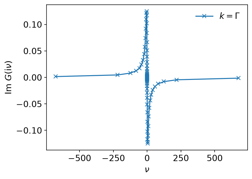
The coefficients fall off like the singular values, which is the statement that the basis is the right one for this function:
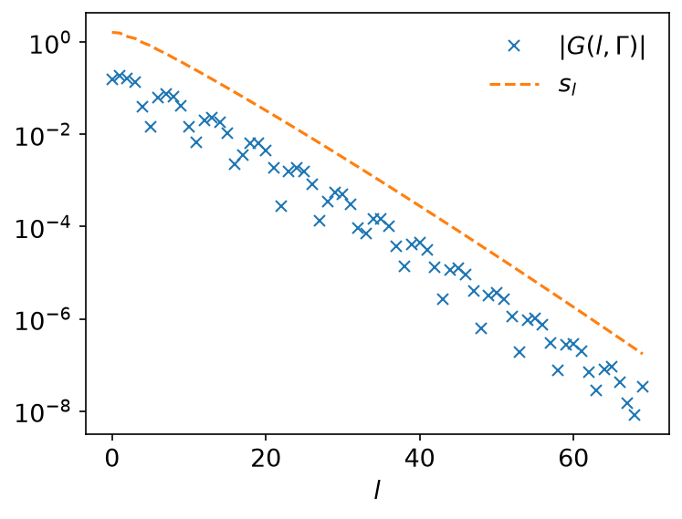
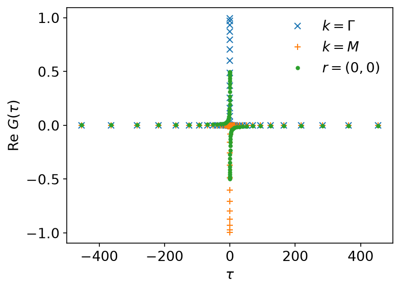
Note where the sampling times lie: on \([-\beta/2, \beta/2]\), not on \([0, \beta)\) as in the Python notebook. The two are the same set of points seen through \(G(\tau - \beta) = -G(\tau)\); see Conventions.
The self-energy
\(G(\beta - \tau)\) is where that convention has to be handled rather than
just noted. On \([0, \beta)\) it is the reversed array, which is what the
notebook writes as grt[::-1]. On the symmetric grid the reversed array is
\(G(-\tau)\), and
\[ G(\beta - \tau) = \zeta, G(-\tau), \qquad \zeta = -1 \text{ (fermionic)},\ +1 \text{ (bosonic)}, \]
so the sign has to come along. IrMesh::reverse_tau is exactly that
operation, and it is the only place in the applied tutorials where the
relation appears. It does not assume the grid is closed under
\(\tau \to -\tau\): a sampling time may sit at exactly \(\beta/2\), whose
mirror is the same point one period away, and the extra \(\zeta\) from that
period is applied where it is needed (see GW, whose grid has such a
point):
    // G(β − τ) on the symmetric grid: the reversed rows, times ζ = −1.
    let reversed = mesh.reverse_tau(&grt, nk);
    let srt: Vec<Complex64> = grt
        .iter()
        .zip(&reversed)
        .map(|(g, g_reversed)| U * U * g * g * g_reversed)
        .collect();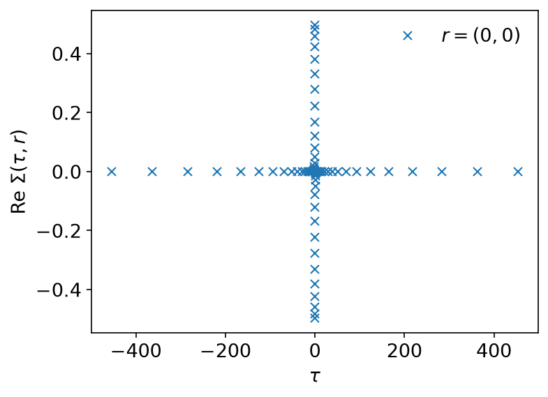
Getting the sign wrong, or reversing without it, changes \(\Sigma\) by a factor of order one — a picture that still looks plausible. So check the relation against a direct evaluation of \(u_l(\beta - \tau)\) rather than trusting a reading of the convention.
Back to the Matsubara axis
The way back is the way in, in reverse:
    let srl = mesh.tau_to_l(&srt, nk)?; // values → coefficients
    let skl = grid.r_to_k(&srl); // and back to momentum
    let sigma_iv = mesh.l_to_wn(&skl, nk)?;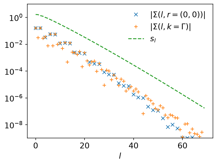
The coefficients of \(\Sigma\) decay like those of \(G\), which says the product of three Green’s functions is still a function the basis represents well — the fact the whole method rests on.
Because the answer is a set of coefficients, \(\Sigma\) can be evaluated on any frequencies at all, not only on the ones that were sampled. Here on every twentieth fermionic frequency out to \(|n| \approx 20000\): the textbook index \(m\) runs in steps of 20, so the reduced index \(n = 2m + 1\) runs in steps of 40, from \(-19999\) to \(19961\).
    // The coefficients are the whole answer: Σ can be evaluated on any
    // frequency, not only on the ones that were sampled. Here, every twentieth
    // fermionic frequency (m in steps of 20, so n = 2m + 1 in steps of 40) out
    // to |n| ≈ 20000 — far beyond the sampling set.
    let far: Vec<i64> = (-10000..10000).step_by(20).map(|n| 2 * n + 1).collect();
    let freqs: Vec<FermionicFreq> = far
        .iter()
        .map(|&n| FermionicFreq::new(n))
        .collect::<Result<_, _>>()?;
    let sampling = MatsubaraSampling::<Fermionic>::with_sampling_points(&basis, freqs)?;
    // Only Γ is wanted, so evaluate one column rather than all of them.
    let skl_gamma: Vec<Complex64> = (0..basis.size()).map(|l| skl[l * nk + gamma]).collect();
    let sigma_far = sampling.evaluate(&skl_gamma)?;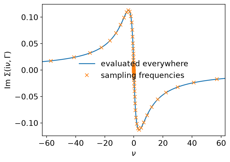
The sampled points lie on the evaluated curve, which is the whole claim: 70 numbers per momentum hold the frequency dependence of \(\Sigma\) everywhere.
Going further
This page uses only the IR basis and stays on the imaginary axis. For real-frequency output, see MiniPole, which fits a few poles to Matsubara data by ESPRIT, and Analytic continuation for why that step is ill posed. The DLR page shows the pole-based representation of imaginary-axis data.
Running it
From docs/tutorial-code:
$ cargo run --release --bin second_order_perturbation
The program writes CSV tables to docs/tutorial-code/data/second_order_perturbation/.
The figures are drawn from those tables; from the repository root, run
uv run --project docs/plotting python docs/plotting/second_order_perturbation_plot.py.
The reversal behind IrMesh::reverse_tau and reverse_tau_as
(reverse_tau_rows) is checked against a direct evaluation of
\(u_l(\beta - \tau)\) in docs/tutorial-code/tests/tau_convention.rs.
Key API pieces
From sparse-ir:
| What you want | What to call |
|---|---|
| values at the sampling frequencies → coefficients | MatsubaraSampling::fit_nd |
| coefficients → values at the sampling times | TauSampling::evaluate_nd_zz |
| the same, for a whole array of momenta | the _nd variants, with the momentum axis as the columns |
| \(\Sigma\) on frequencies you choose | MatsubaraSampling::with_sampling_points |
From the tutorial crate (sparse_ir_tutorial, not part of the library):
| What you want | What to call |
|---|---|
| both samplings of one basis, applied to a block of columns | IrMesh::wn_to_l, l_to_tau, tau_to_l, l_to_wn |
| \(G(\beta - \tau)\) on the symmetric grid | IrMesh::reverse_tau (reverse the rows, apply \(\zeta\)) |
| FFTs between momentum and real space | MomentumGrid::k_to_r, r_to_k |
The _nd variants are what keep this example fast: one call moves all 65536
momenta between representations, where a loop over evaluate would pay the
setup cost 65536 times.
GW
Ported from the Python notebook
GW_py.ipynb
of sparse-ir-tutorial.
The program that produced every number and figure on this page is
docs/tutorial-code/src/bin/gw.rs; the code below is included from it.
The previous page evaluated one diagram once. This one runs a self-consistent loop, and in doing so moves between imaginary time, IR coefficients and Matsubara frequencies several times per iteration, in both statistics. It uses the IR basis only.
The parameters are \(T = 0.1\) (\(\beta = 10\)), \(\omega_\mathrm{max} = 1\), \(U = 0.5\), the default accuracy of the basis, and twenty iterations. The non-interacting \(G_0\) has a semicircular spectral function of half-width 1.
Theory
The loop follows the structure of Hedin’s equations in the \(GW\) approximation, for a single site with a bare interaction \(U\). In the notebook’s conventions, which this port keeps, they read
\[ P(\tau) = G(\tau), G(\beta - \tau), \qquad W(\mathrm{i}\omega) = \frac{U}{1 - U P(\mathrm{i}\omega)}, \qquad \Sigma(\tau) = G(\tau), W(\tau), \]
closed by the Dyson equation \(G^{-1} = G_0^{-1} - \Sigma\). Each of them is diagonal in exactly one representation: the two products live in imaginary time, the screening is algebraic on the Matsubara axis, and so is the Dyson equation. One iteration is therefore a tour:
G(iν) → g_l → G(τ) → P(τ) → P_l → P(iω) → W(iω) → W_l → W(τ) → Σ(τ) → Σ_l → Σ(iν) → G(iν)
Here \(\mathrm{i}\nu\) is fermionic and \(\mathrm{i}\omega\) bosonic.
These signs are not the textbook ones. Since \(G(\tau) \le 0\) on \((0, \beta)\), \(P(\tau) = G(\tau) G(\beta - \tau)\) is positive; it is minus the usual single-spin bubble \(G(\tau) G(-\tau)\). The textbook self-energy is \(\Sigma = -GW\), with a spin sum in \(P\). The two sign changes cancel at order \(U^2\), so the second-order term has the textbook sign; the higher-order terms of the screening series do not. The example is about the structure of the loop — which product lives in which representation — not a quantitatively faithful \(GW\) for this model.
Only the constant part of \(W\) is split off: what is carried into
\(\Sigma\) is \(U/(1 - UP) - U\). The instantaneous part \(U\) would
give the static term \(U G(\beta^-) = -U\langle n \rangle\), with
\(\langle n\rangle\) the occupation per spin. In Hedin’s equations that is
the exchange (Fock) term, not the Hartree term; the code calls it hartree
after the notebook. It is computed separately and kept out of the Dyson
equation, because a constant only shifts the chemical potential.
Two statistics, one loop
\(G\) and \(\Sigma\) are fermionic; \(P\) and \(W\) are bosonic. The two products mix them: \(P\) is a product of \(G\)’s evaluated at the bosonic sampling times, and \(\Sigma\) needs \(W\) at the fermionic ones. So the example carries two bases and two meshes:
    // Two bases with the same Λ = βω_max. `new` runs the SVE for each; for a
    // larger Λ, compute it once and use `FiniteTempBasis::from_sve_result`.
    let basis_f = FiniteTempBasis::<LogisticKernel, Fermionic>::new(
        LogisticKernel::new(BETA * WMAX)?,
        BETA,
        None,
        None,
    )?;
    let basis_b = FiniteTempBasis::<LogisticKernel, Bosonic>::new(
        LogisticKernel::new(BETA * WMAX)?,
        BETA,
        None,
        None,
    )?;
    let mesh_f = IrMesh::<Fermionic>::new(&basis_f)?;
    let mesh_b = IrMesh::<Bosonic>::new(&basis_b)?;
Both bases use the same kernel, so they could share one singular value
expansion. Calling FiniteTempBasis::new twice computes it twice; at
\(\Lambda = 10\) that costs nothing, but for a large \(\Lambda\) compute the
SVE once and build both bases with FiniteTempBasis::from_sve_result, as
Conventions shows.
The loop also needs two evaluation matrices, built once outside it, and the row \(u_l(\beta^-)\) for the static term:
    // The two cross-statistics evaluation matrices, built once: the fermionic
    // basis functions at the bosonic sampling times, and the other way round.
    let uf_at_tau_b = basis_f.evaluate_tau(mesh_b.tau_points())?;
    let ub_at_tau_f = basis_b.evaluate_tau(mesh_f.tau_points())?;
    // u_l(β⁻), for the Hartree term.
    let uf_at_beta = basis_f.evaluate_tau(&[BETA])?;
Basis::evaluate_tau is the operation that makes this safe. The sampling
times live on \([-\beta/2, \beta/2]\), so evaluating a basis function there
needs the (anti-)periodicity relation — and which relation is a property of
the function, never of the grid it is being sampled on. \(G\) stays
anti-periodic when evaluated at bosonic times; \(W\) stays periodic at
fermionic ones. evaluate_tau applies the statistics of the basis it belongs
to, which is exactly right. Doing the same thing by hand — folding the times
and then multiplying by a sign taken from the grid — is the mistake this
example exists to rule out.
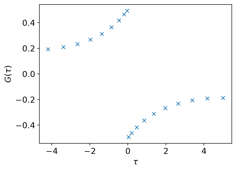
The reversal, again
\(P(\tau) = G(\tau) G(\beta - \tau)\) needs the same reversal as the second-order self-energy, and here it has a wrinkle. At \(\beta = 10\), \(\omega_\mathrm{max} = 1\) and the default accuracy, both grids hold 19 points: 18 of them in \(\pm\) pairs, and one at exactly \(\tau = \beta/2\). That last point has no partner under \(\tau \to -\tau\) on the grid — its mirror \(-\beta/2\) is the same point one period away. The reversal must therefore allow for a wrap, which brings a second \(\zeta\); at \(\beta/2\) the two cancel and the row maps to itself with a plus sign.
evaluate_rows (a tutorial helper) contracts a matrix of basis-function
values with a block of coefficients:
        let g_tau_b = evaluate_rows(&uf_at_tau_b, &g_l_f, 1);
        // P(τ) = G(τ) G(β − τ), with G(β − τ) = −G(−τ): the reversed array
        // with the *fermionic* sign, even though the times are the bosonic
        // ones. This grid also carries a point at exactly τ = β/2, whose
        // mirror is itself one period away; `reverse_tau_as` handles that.
        let g_beta_minus_tau = mesh_b.reverse_tau_as::<Fermionic>(&g_tau_b, 1);
        let p_tau_b: Vec<Complex64> = g_tau_b
            .iter()
            .zip(&g_beta_minus_tau)
            .map(|(g, g_reversed)| g * g_reversed)
            .collect();
        let p_l_b = mesh_b.tau_to_l(&p_tau_b, 1)?;
        let p_iw_b = mesh_b.l_to_wn(&p_l_b, 1)?;
For this particular model the check is worth stating plainly: the model is particle-hole symmetric, so \(G(\beta - \tau) = G(\tau)\) and a plot of the two would show one curve. The fermionic and bosonic sampling times coincide as well, because the logistic kernel gives both statistics the same \(u_l(\tau)\). Neither the picture nor the abscissa would reveal a missing \(\zeta\) — only the numbers would.
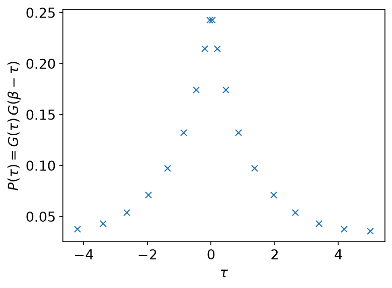
The screened interaction
\(W\) is algebraic on the Matsubara axis and then has to come back to imaginary time — on the fermionic grid, because that is where it meets \(G\):
        // W = U/(1 − UP); only the frequency-dependent part U/(1 − UP) − U is
        // carried on, the constant being the bare interaction itself.
        let w_iw_b: Vec<Complex64> = p_iw_b.iter().map(|p| U / (1.0 - U * p) - U).collect();
        let w_l_b = mesh_b.wn_to_l(&w_iw_b, 1)?;
        // --- and back into fermionic statistics -------------------------------
        let w_tau_f = evaluate_rows(&ub_at_tau_f, &w_l_b, 1);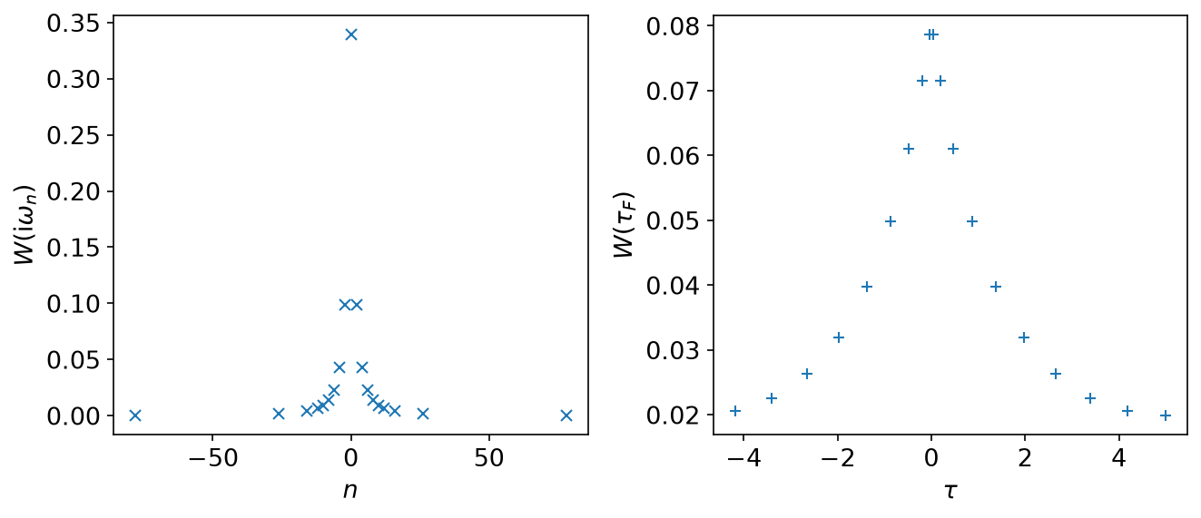
The self-energy, and the loop
        let e_tau_f: Vec<Complex64> = g_tau_f.iter().zip(&w_tau_f).map(|(g, w)| g * w).collect();
        let e_l_f = mesh_f.tau_to_l(&e_tau_f, 1)?;
        let e_iw_f = mesh_f.l_to_wn(&e_l_f, 1)?;
        // The static term U G(β⁻) = −U⟨n⟩. The name follows the notebook; in
        // Hedin's equations this instantaneous piece is the exchange (Fock)
        // term. It is subtracted, so the reported Σ carries +U⟨n⟩.
        let hartree: Complex64 = U * evaluate_rows(&uf_at_beta, &g_l_f, 1)[0];
        let e_iw_f_hartree: Vec<Complex64> = e_iw_f.iter().map(|e| e - hartree).collect();
and the Dyson equation \(G = 1/(G_0^{-1} - \Sigma)\) closes the loop:
        // The Dyson equation. The static term is left out of it, as in the
        // notebook: it is a constant shift of the chemical potential.
        g_iw_f = g_iw_0
            .iter()
            .zip(&e_iw_f)
            .map(|(g0, e)| (g0.inv() - e).inv())
            .collect();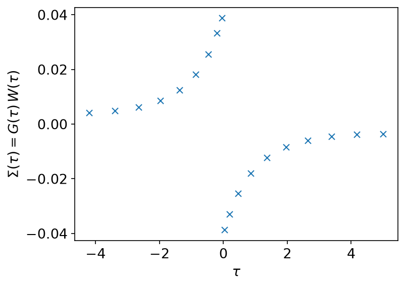
Both expansions fall off like the singular values of their own basis, which is the statement that a product of Green’s functions is still a function the basis represents well — the fact the whole method rests on:
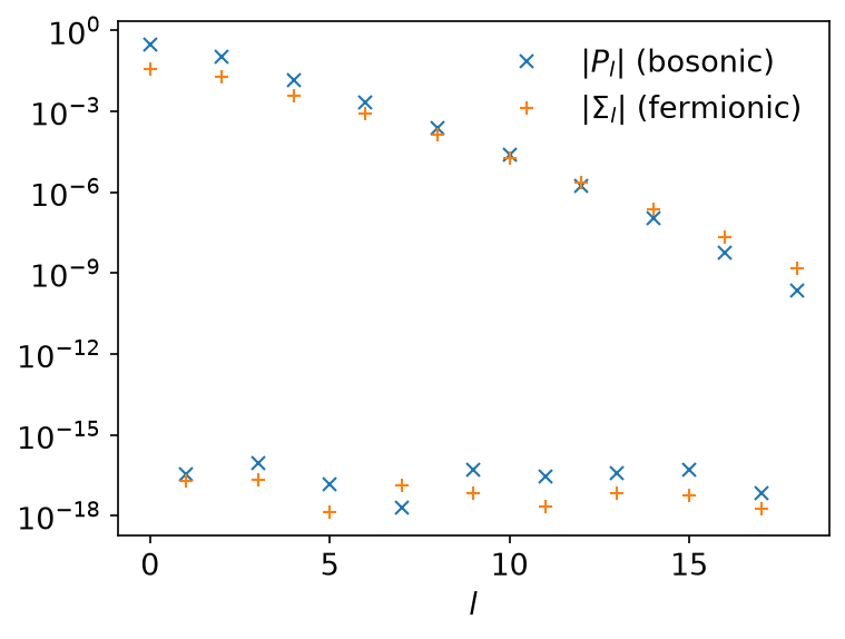
Twenty iterations are more than enough: the change in \(\Sigma\) falls by about a decade per step and reaches the rounding floor around iteration 18.
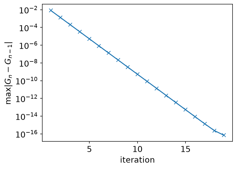
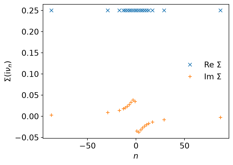
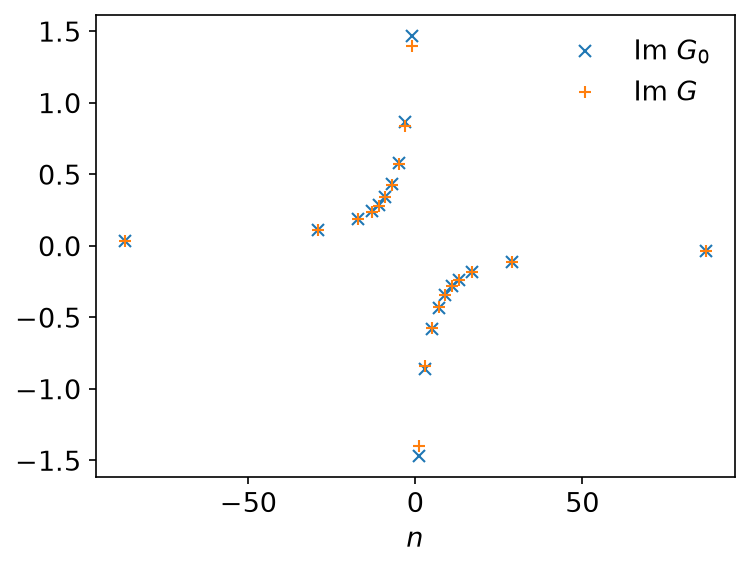
Going further
This page uses only the IR basis and stays on the imaginary axis. For real-frequency output, see MiniPole, which fits a few poles to Matsubara data by ESPRIT, and Analytic continuation for why that step is ill posed. The DLR page shows the pole-based representation of imaginary-axis data.
Running it
From docs/tutorial-code:
$ cargo run --release --bin gw
The program writes CSV tables to docs/tutorial-code/data/gw/. The figures
are drawn from those tables; from the repository root, run
uv run --project docs/plotting python docs/plotting/gw_plot.py. The reversal behind IrMesh::reverse_tau and reverse_tau_as
(reverse_tau_rows) is checked against a direct evaluation of
\(u_l(\beta - \tau)\) in docs/tutorial-code/tests/tau_convention.rs.
Key API pieces
From sparse-ir:
| What you want | What to call |
|---|---|
| a basis function of one statistics at the other’s sampling times | Basis::evaluate_tau |
| \(u_l(\beta^-)\), for the static term | Basis::evaluate_tau(&[beta]) |
| two bases from one SVE | compute_sve, then FiniteTempBasis::from_sve_result |
From the tutorial crate (sparse_ir_tutorial, not part of the library):
| What you want | What to call |
|---|---|
| \(G(\beta - \tau)\) for a function whose statistics is not the mesh’s | IrMesh::reverse_tau_as::<S> |
| the round trip through the basis | IrMesh::wn_to_l, l_to_tau, tau_to_l, l_to_wn |
| a matrix of basis-function values times a block of coefficients | evaluate_rows |
The whole loop is 19 + 19 coefficients wide. Nothing in it ever sees a dense imaginary-time grid.
Exchange interactions
Ported from the Python notebook
liechtenstein_py.ipynb
of sparse-ir-tutorial,
whose author is Takuya Nomoto. The program that produced every number and
figure on this page is docs/tutorial-code/src/bin/liechtenstein.rs; the code
below is included from it.
Both previous applied pages used the basis to hold a function of imaginary time. This one uses it for something narrower and, in its way, more striking: to do a Matsubara sum in one evaluation.
Theory
The Liechtenstein method reads the parameters of a classical spin model off an itinerant one by requiring that the two have the same second derivative of the total energy with respect to spin angles. For a single orbital,
\[ H = -t \sum_{\langle i, j\rangle, s} c^\dagger_{is} c_{js}
- \sum_i \sum_{ss’} c^\dagger_{is} (\boldsymbol{B}i \cdot \boldsymbol{\sigma}{ss’}) c_{is’}, \]
expanded about the ferromagnetic state \(\boldsymbol{B}_i = B\hat{z}\), the requirement gives
\[ J_{ij} = -B^2 T \sum_\nu G_{ij,+}(\mathrm{i}\nu) G_{ji,-}(\mathrm{i}\nu), \]
and, for the quantity that sets the mean-field transition temperature \(T_c^\mathrm{mf} = 2J_0/3\),
\[ J_0 = \frac{B}{2}(n_{0,+} - n_{0,-}) + B^2 T \sum_\nu G_{00,+}(\mathrm{i}\nu) G_{00,-}(\mathrm{i}\nu). \]
Here \(G_{ij,\pm}\) is the Green’s function of spin \(\pm\) in the field, and \(\nu = \nu_n = n\pi/\beta\) runs over all fermionic frequencies (\(n\) odd). Both are Matsubara sums of a product of two Green’s functions. That product falls off as \(1/\nu^2\), so a truncated sum converges like \(1/N_M\) — slowly, and the more slowly the colder the system.
Parameters
The example uses a square lattice with nearest-neighbour hopping \(t = 1\) on a \(36 \times 36\) momentum grid, the field \(B = 3\), \(\beta = 50\) and \(\varepsilon = 10^{-7}\). \(J_0\) is scanned over 41 chemical potentials from \(\mu = -10\) to \(10\); \(J_{ij}\) is computed at half filling, \(\mu = 0\). The basis has to hold both spin-split bands, so \(\omega_\mathrm{max} = 2 \max(W, B) = 16\) with the bandwidth \(W = 8t\), and \(\Lambda = \beta\omega_\mathrm{max} = 800\).
const T_HOPPING: f64 = 1.0;
const BETA: f64 = 50.0;
const NK_LIN: usize = 36;
/// The effective field that polarizes the reference state.
const B_EFF: f64 = 3.0;
const EPS: f64 = 1e-7;
/// `2 max(W, B) β` with the bandwidth `W = 8t`: the basis has to hold the
/// whole of both spin-split bands.
const LAMBDA: f64 = 2.0 * 8.0 * T_HOPPING * BETA;
/// How many chemical potentials `J₀` is scanned over, from −10 to 10.
const N_MU: usize = 41;
/// The truncated Matsubara grids `J₀` is also evaluated on, for comparison.
const NAIVE: [usize; 5] = [100, 200, 400, 800, 1600];
The sum as an evaluation
The way out is the elementary identity
\[ T \sum_\nu F(\mathrm{i}\nu) = F(\tau = 0), \]
which turns the sum into one point of the imaginary-time function behind it. A product of two Green’s functions is as representable in the basis as a single one, so the whole sum costs a fit and one evaluation:
    // `T Σ_ν F(iν) = F(τ = 0)`: the Matsubara sum is the basis expansion read
    // at one point. This is the row of basis functions that reads it.
    let u_at_zero = basis.evaluate_tau(&[0.0])?;
    let occupation = occupation_term(&ek, &mu);
    // One column per chemical potential, one row per sampling frequency.
    let mut sampled = Vec::with_capacity(mesh.n_wn() * N_MU);
    for freq in mesh.wn() {
        sampled.extend(product_at(freq.value(BETA), &ek, &mu));
    }
    let coefficients = mesh.wn_to_l(&sampled, N_MU)?;
    let summed = evaluate_rows(&u_at_zero, &coefficients, N_MU);
    let j0: Vec<f64> = occupation
        .iter()
        .zip(&summed)
        .map(|(n, s)| n + s.re)
        .collect();
sampled holds the product at the 38 sampling frequencies, one column per
chemical potential; evaluate_rows (a tutorial helper) contracts the
coefficients with \(u_l(0)\). At \(\beta = 50\) and \(\Lambda = 800\)
the basis has 37 functions. The size grows only like \(\log \beta\): since
\(\Lambda = 16t\beta\) here, \(\beta = 500\) gives 53 functions and
\(\beta = 5000\) gives 68, for a hundred times lower temperature.
The example also sums the series the naive way, on symmetric grids of 200 to 3200 frequencies (100 to 1600 on each side of zero), so that the two can be put side by side:
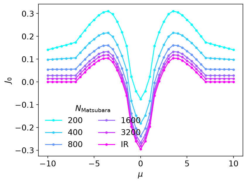
The truncated sums are above the converged answer everywhere and creep down towards it. How fast is the whole story:
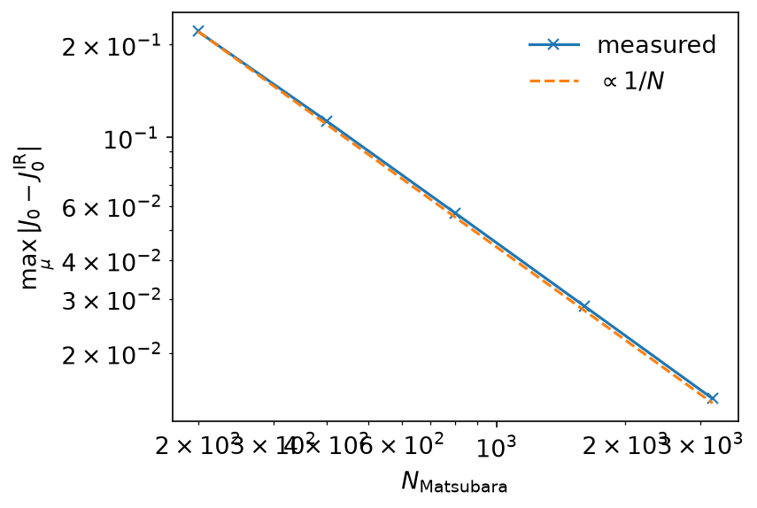
Halving the error costs a doubling of the grid. Reaching the basis answer that way would take of order \(10^{9}\) frequencies; the basis reaches it with 38.
The physics, once the answer is trusted: \(J_0 < 0\) at half filling, where the system is an antiferromagnet by super-exchange, and \(J_0 > 0\) in the low-carrier regime, where double exchange makes it a ferromagnet.
\(J_{ij}\), and a check
\(J_{ij}\) needs the Green’s function in real space rather than its zone average, so a Fourier transform joins the sum. \(G_{ij}\) carries \(e^{-\mathrm{i}k\cdot r}\) and \(G_{ji}\) carries \(e^{+\mathrm{i}k\cdot r}\); since \(\epsilon_{\boldsymbol{k}}\) is even, the second is the first applied to the same array. The program checks that before relying on it:
    assert!(
        (0..grid.len()).all(|index| {
            let (k1, k2) = (index / NK_LIN, index % NK_LIN);
            let mirrored = ((NK_LIN - k1) % NK_LIN) * NK_LIN + (NK_LIN - k2) % NK_LIN;
            (ek[index] - ek[mirrored]).abs() < 1e-12
        }),
        "the dispersion must be even in k for G_ji to be the transform of G_ij"
    );
The on-site term \(J_{00}\) is not an exchange interaction, so it is set to zero:
    // The on-site term is not an exchange interaction; the notebook drops it.
    jij[0] = 0.0;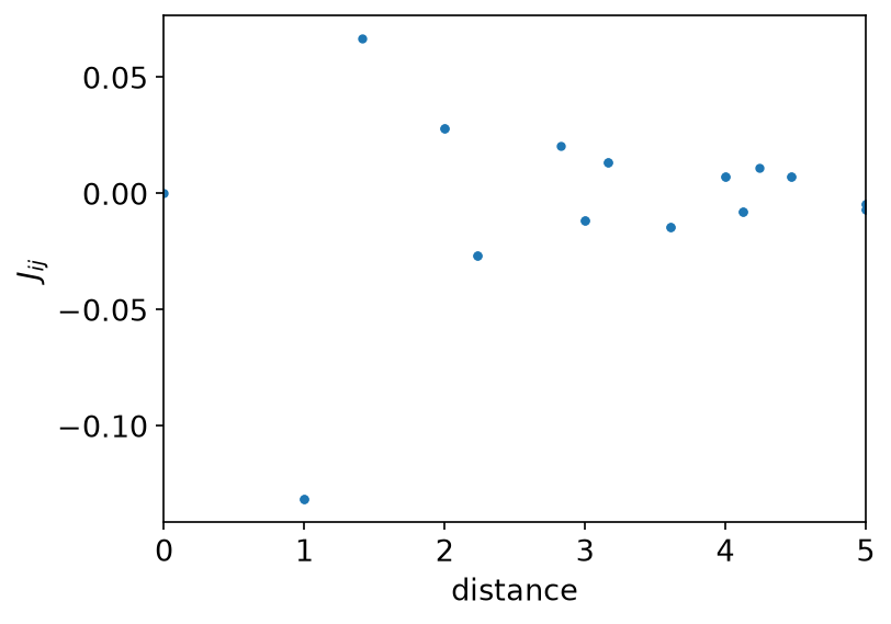
The sum rule \(J_0 = \sum_{j \ne 0} J_{0j}\) then connects the two calculations, which took different routes: one never left momentum space, the other summed the 1295 off-site terms of the \(36 \times 36\) real-space lattice. At \(\mu = 0\) they agree to \(4 \times 10^{-8}\) (\(J_0 \approx -0.2954590\)), which is the accuracy of the basis (\(\varepsilon = 10^{-7}\)) and not machine precision — as it should be.
Going further
This page uses only the IR basis and stays on the imaginary axis. For real-frequency output, see MiniPole, which fits a few poles to Matsubara data by ESPRIT, and Analytic continuation for why that step is ill posed. The DLR page shows the pole-based representation of imaginary-axis data.
Running it
From docs/tutorial-code:
$ cargo run --release --bin liechtenstein
The program writes CSV tables to docs/tutorial-code/data/liechtenstein/. The
figures are drawn from those tables; from the repository root, run
uv run --project docs/plotting python docs/plotting/liechtenstein_plot.py.
Key API pieces
From sparse-ir:
| What you want | What to call |
|---|---|
| a Matsubara sum | fit (MatsubaraSampling::fit_nd), then evaluate at τ = 0 |
| the row \(u_l(0)\) | Basis::evaluate_tau(&[0.0]) |
From the tutorial crate (sparse_ir_tutorial, not part of the library):
| What you want | What to call |
|---|---|
| many chemical potentials at once | one column each; IrMesh::wn_to_l takes them together |
| contract \(u_l(0)\) with a block of coefficients | evaluate_rows |
| FFT from momentum to real space | MomentumGrid::k_to_r |
Orbital magnetic susceptibility
Ported from the Python notebook
orbital_magnetic_susceptibility_py.ipynb
of sparse-ir-tutorial,
whose authors are Soshun Ozaki and Takashi Koretsune. The program that
produced every number and figure on this page is
docs/tutorial-code/src/bin/orbital_magnetic_susceptibility.rs; the code below
is included from it.
The previous page used the basis to turn a Matsubara sum into one evaluation. This one does the same thing for a harder summand, and adds the other piece every multi-orbital calculation needs: a Hamiltonian that is a matrix at each momentum.
Theory
Orbital magnetism is what a vector potential coupled to the electron momentum induces. For a tight-binding model the susceptibility has a closed form in terms of the Green’s function and the derivatives of the Hamiltonian,
\[ \chi = T \sum_\nu \chi(\mathrm{i}\nu), \qquad \chi(\mathrm{i}\nu) = \frac{1}{N_k}\sum_{\boldsymbol{k}} \mathrm{Tr}\left[ \gamma_x G \gamma_y G \gamma_x G \gamma_y G
- \tfrac{1}{2}(\gamma_x G \gamma_y G + \gamma_y G \gamma_x G)\gamma_{xy} G \right], \]
with \(G = G(\mathrm{i}\nu, \boldsymbol{k})\), \(\gamma_i = \partial H_{\boldsymbol{k}} / \partial k_i\), \(\gamma_{xy} = \partial^2 H_{\boldsymbol{k}} / \partial k_x \partial k_y\), and \(\nu = \nu_n = n\pi/\beta\) running over the fermionic frequencies (\(n\) odd). The momentum sum is an average over the \(N_k\) points of the zone, so \(\chi\) is per unit cell. Units are \(e = \hbar = k_B = 1\) with \(t = a = 1\): the prefactor \(e^2/\hbar^2\) of the notebook’s formula is dropped. No spin factor is included, so \(\chi\) is for one spin species; multiply by 2 for spin-degenerate electrons. The formula is due to Gómez-Santos and Stauber, and to Raoux, Piéchon, Fuchs and Montambaux; its relation to Fukuyama’s continuum formula was settled by Ogata and Fukuyama and by Matsuura and Ogata.
The example computes it at \(T = 0.1\) (\(\beta = 10\)) on a \(200 \times 200\) momentum grid, for 91 chemical potentials from \(\mu = -4.5\) to \(4.5\). The basis uses \(\omega_\mathrm{max} = 10\) (\(\Lambda = 100\)) and \(\varepsilon = 10^{-10}\), which gives 30 functions:
const T_HOPPING: f64 = 1.0;
const LATTICE: f64 = 1.0;
const TEMPERATURE: f64 = 0.1;
const BETA: f64 = 1.0 / TEMPERATURE;
const WMAX: f64 = 10.0;
const EPS: f64 = 1e-10;
const NK_LIN: usize = 200;
/// The chemical potentials `χ` is scanned over, from −4.5 to 4.5.
const N_MU: usize = 91;
const MU_MIN: f64 = -4.5;
const MU_MAX: f64 = 4.5;
/// The chemical potential the sampled `χ(iν)` is written out at. Not μ = 0:
/// both lattices are particle-hole symmetric there and `χ(iν)` comes out
/// real, which would hide a mistake in its imaginary part.
const PROBE_MU: f64 = -1.0;
It is written entirely in Matsubara sums of products of Green’s functions, which is what makes it a good example. Here the summand is a product of three or four of them, not two:
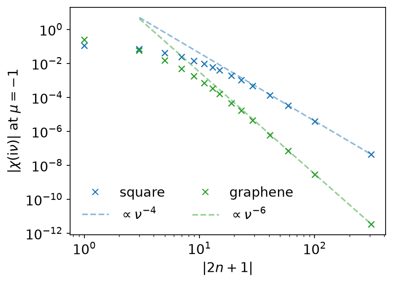
The square lattice falls off as \(\nu^{-4}\) — a dispersion that separates has no \(\gamma_{xy}\), so the three-Green’s-function term is absent entirely — and graphene, whose velocity matrices are purely off-diagonal in the site basis, as \(\nu^{-6}\). Thirty sampling frequencies hold all of it, and the sum is again
    // `T Σ_ν F(iν) = F(τ = 0)`: the Matsubara sum is the basis expansion read
    // at one point. This is the row of basis functions that reads it.
    let u_at_zero = basis.evaluate_tau(&[0.0])?;
        let coefficients = mesh.wn_to_l(&chi_iw, N_MU)?;
        let chi: Vec<f64> = evaluate_rows(&u_at_zero, &coefficients, N_MU)
            .iter()
            .map(|z| z.re)
            .collect();
with one column per chemical potential; there are 91 of them, fitted in one call.
Square lattice
One band makes every matrix in the formula a number and the trace a product, so the whole summand is two terms:
        for (i, &nu) in nu.iter().enumerate() {
            for (m, &mu) in mu.iter().enumerate() {
                let g = Complex64::new(-(ek - mu), nu).inv();
                let g2 = g * g;
                chi[i * n_mu + m] += gx * gx * gy * gy * g2 * g2 + gx * gy * gxy * g2 * g;
            }
        }
After the loop over momenta, the sum is divided by \(N_k\):
    // The k sum is an average over the zone: χ per unit cell.
    let nk = grid.len() as f64;
    chi.iter().map(|z| z / nk).collect()
\(\gamma_{xy}\) is identically zero here, and the second term with it; the example keeps it so that the code is the formula rather than a special case of it.
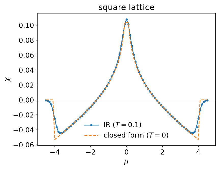
At \(T = 0\) the same quantity is known in closed form,
\[ \chi = -\frac{2}{3\pi^2}\left[E(m) - \frac{K(m)}{2}\right], \qquad m = 1 - \frac{\mu^2}{16}, \]
zero outside the band. sparse_ir_tutorial::elliptic computes \(K\) and
\(E\) from the arithmetic-geometric mean, which is a dozen lines and needs
no dependency. The two curves lie on top of each other to better than
\(10^{-3}\) for \(1 \le |\mu| \le 3\), and part company only where they
must: at the van Hove filling \(\mu = 0\), where the closed form diverges and
\(T = 0.1\) does not, and at the band edge, where the Fermi function rounds
the step off. Because of the divergence, the program leaves \(\mu = 0\) out of
the closed-form table.
Graphene
Two sites per cell make \(H_{\boldsymbol{k}}\) a 2×2 matrix, which has to be diagonalised before the Green’s function can be written down. In the eigenbasis \(G\) is diagonal, so the trace of four matrices becomes a product of 2×2 matrices whose columns are scaled by \(G\):
        let eigen = hamiltonian.eigen();
        // In the eigenbasis `G` is diagonal, so the traces below are products
        // of 2×2 matrices and two numbers rather than of four matrices.
        let [gx, gy, gxy] = velocities.map(|m| Hermitian2::rotate(&eigen, &m));
        for (i, &nu) in nu.iter().enumerate() {
            for (m, &mu) in mu.iter().enumerate() {
                let g = [
                    Complex64::new(-(eigen.values[0] - mu), nu).inv(),
                    Complex64::new(-(eigen.values[1] - mu), nu).inv(),
                ];
                let (xg, yg, xyg) = (
                    times_green(&gx, &g),
                    times_green(&gy, &g),
                    times_green(&gxy, &g),
                );
                let xy = product(&xg, &yg);
                let yx = product(&yg, &xg);
                chi[i * n_mu + m] += trace(&xy, &xy) + 0.5 * (trace(&xy, &xyg) + trace(&yx, &xyg));
            }
        }
Hermitian2 in sparse_ir_tutorial::linalg solves the 2×2 eigenproblem in
closed form rather than calling a general routine, because a general routine
is free to return the eigenvectors with any phase and the tutorial’s numbers
have to be reproducible. The susceptibility does not care about the phase:
it is a trace of rotated matrices.
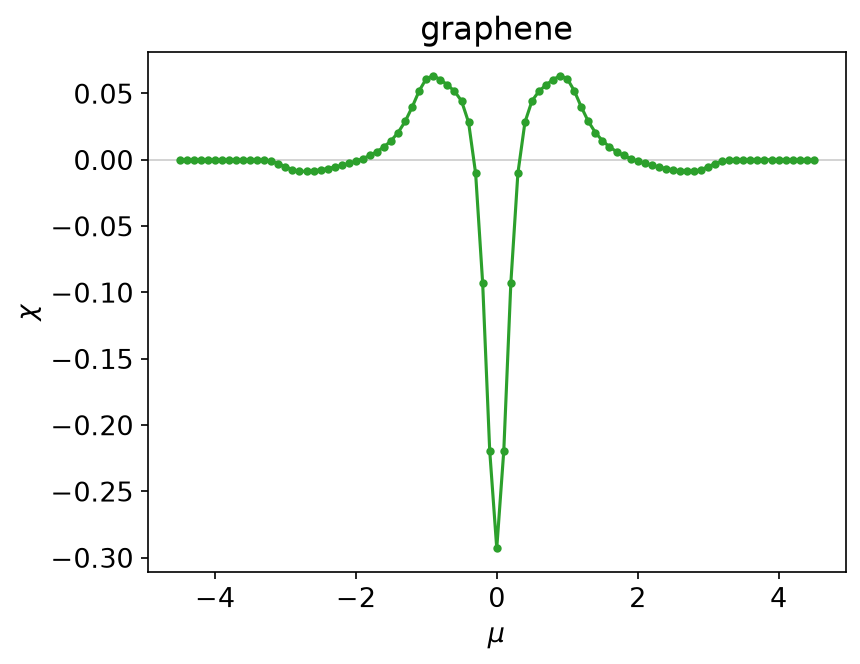
The result is the opposite of the square lattice: a sharp diamagnetic peak at the Dirac point, the delta function of the massless spectrum rounded by temperature, paramagnetic shoulders on either side, and nothing at all outside the band, which spans \(|\epsilon| \le 3t\).
Going further
This page uses only the IR basis and stays on the imaginary axis. For real-frequency output, see MiniPole, which fits a few poles to Matsubara data by ESPRIT, and Analytic continuation for why that step is ill posed. The DLR page shows the pole-based representation of imaginary-axis data.
Running it
From docs/tutorial-code:
$ cargo run --release --bin orbital_magnetic_susceptibility
The program writes CSV tables to
docs/tutorial-code/data/orbital_magnetic_susceptibility/. The figures are
drawn from those tables; from the repository root, run
uv run --project docs/plotting python docs/plotting/orbital_magnetic_susceptibility_plot.py.
The Python counterpart of this program,
docs/tutorial-code/scripts/reference_orbital_magnetic_susceptibility.py,
diagonalises with numpy’s eigh, which picks other eigenvector phases; the
susceptibilities of the two agree to about
\(2 \times 10^{-14}\).
Key API pieces
From sparse-ir:
| What you want | What to call |
|---|---|
| a Matsubara sum | fit (MatsubaraSampling::fit_nd), then evaluate at τ = 0 |
| the row \(u_l(0)\) | Basis::evaluate_tau(&[0.0]) |
From the tutorial crate (sparse_ir_tutorial, not part of the library):
| What you want | What to call |
|---|---|
| many chemical potentials at once | one column each; IrMesh::wn_to_l takes them together |
| contract \(u_l(0)\) with a block of coefficients | evaluate_rows |
| a 2×2 Hermitian eigenproblem | Hermitian2::eigen, Hermitian2::rotate |
| \(K(m)\), \(E(m)\) | elliptic::ellipk, elliptic::ellipe |
DMFT with an IPT solver
Ported from the Python notebook
DMFT_IPT_py.ipynb
of the sparse-ir tutorials,
whose author is Niklas Witt. The programs that produced every number and
figure on this page are docs/tutorial-code/src/bin/dmft_ipt.rs and
docs/tutorial-code/src/bin/dmft_ipt_scan.rs; the loop itself is in
docs/tutorial-code/src/dmft.rs, and the code below is included from there.
Every applied page so far computed something once. This one iterates: a self-consistency loop that goes through the basis twice per step, several thousand times over. That makes it the page where the basis has to be cheap, and the page where a symmetry the exact solution has, but the arithmetic only nearly has, decides what the loop converges to.
The model and the loop
Dynamical mean-field theory replaces a lattice problem by a single impurity in a bath that is fixed by demanding that the impurity’s Green’s function is the lattice’s local one. On the Bethe lattice, with the semicircular density of states
\[ \rho(\omega) = \frac{2}{\pi D^2}\sqrt{D^2 - \omega^2}, \qquad D = 2t_\star = 2, \]
the self-consistency condition collapses to one line,
\[ \mathcal{G}^{-1}(\mathrm{i}\nu) = \mathrm{i}\nu - t_\star^2 G_\mathrm{loc}(\mathrm{i}\nu), \]
and iterated perturbation theory approximates the impurity self-energy by the second-order diagram, which at half filling is just a cube in imaginary time:
\[ \Sigma(\tau) = U^2 \mathcal{G}(\tau)^3, \qquad G_\mathrm{loc}^{-1}(\mathrm{i}\nu) = \mathcal{G}^{-1}(\mathrm{i}\nu) - \Sigma(\mathrm{i}\nu). \]
\(\Sigma\) is local in \(\tau\) and the Dyson equation is local in \(\mathrm{i}\nu\), so each iteration is a round trip between the two representations — exactly what the basis is for:
            // Σ(τ) = U² 𝒢(τ)³, which is the whole impurity solver.
            let g_tau = self.mesh.wn_to_tau(&g_weiss, 1)?;
            let sigma_tau: Vec<Complex64> = g_tau.iter().map(|g| u * u * g * g * g).collect();
            let mut fresh = self.mesh.tau_to_wn(&sigma_tau, 1)?;
At \(\beta = 20\), \(\omega_\mathrm{max} = 2D = 4\) and \(\varepsilon = 10^{-15}\) the basis has 37 functions, with 37 sampling times and 38 sampling frequencies. That is the entire state of the calculation: 37 coefficients carry a function whose Matsubara tail reaches out to \(\nu \sim 10^2\), and the round trip is two small dense solves. Nothing in the loop grows with \(\beta\) except logarithmically, which is what makes a 5000-iteration run a matter of seconds.
The non-interacting starting point comes from the same basis. The spectral representation \(G^0(\mathrm{i}\nu) = \int\mathrm{d}\omega, \rho(\omega)/(\mathrm{i}\nu - \omega)\) becomes, in IR coefficients, \(g_l = -s_l \rho_l\) with \(\rho_l = \int\mathrm{d}\omega, v_l(\omega)\rho(\omega)\). The overlap \(\rho_l\) is computed by Gauss–Legendre quadrature after the substitution \(\omega = D\sin\theta\), which removes the square-root singularity at the band edges, so the result is exact to machine precision:
        let rho_l = shifted_semicircle_overlaps(&self.basis, 0.0, self.d, 1.0);
        let g_l: Vec<Complex64> = self
            .basis
            .s()
            .iter()
            .zip(&rho_l)
            .map(|(s, rho)| Complex64::new(-s * rho, 0.0))
            .collect();
        self.mesh.l_to_wn(&g_l, 1)
The mixing is the notebook’s: \(\Sigma \leftarrow 0.25,\Sigma_\mathrm{new}
- 0.75,\Sigma_\mathrm{old}\).
One step is not in the notebook. At half filling with a symmetric density of states the exact self-energy is particle-hole symmetric: \(\Sigma(\mathrm{i}\nu)\) is purely imaginary and odd in \(\nu\). The round trip through the basis preserves that only to rounding, so the loop projects each new self-energy back onto its symmetric part, \(\Sigma(\mathrm{i}\nu) \to \mathrm{i},\tfrac12[\mathrm{Im},\Sigma(\mathrm{i}\nu) - \mathrm{Im},\Sigma(-\mathrm{i}\nu)]\). The next section shows why that is not optional.
            if symmetry == Symmetry::ParticleHole {
                fresh = self.particle_hole_symmetric(&fresh);
            }
One solve at \(U = 5\)
Run the loop at \(U = 5\) with the notebook’s stopping rule — stop when the relative change of \(\Sigma\) falls below \(10^{-5}\) — and it stops at iteration 65, reporting
\[ Z = \left(1 - \frac{\partial,\mathrm{Im},\Sigma}{\partial \nu}\right)^{-1} \approx 0.263, \]
a quasiparticle weight of a quarter: a correlated metal. The derivative is a finite difference over the two lowest positive frequencies, \(\partial,\mathrm{Im},\Sigma/\partial\nu \approx [\mathrm{Im},\Sigma(\mathrm{i}\nu_3) - \mathrm{Im},\Sigma(\mathrm{i}\nu_1)] /(2\pi/\beta)\) (reduced indices \(n = 1, 3\)), and a negative \(Z\) is reported as zero. Here is that solution:
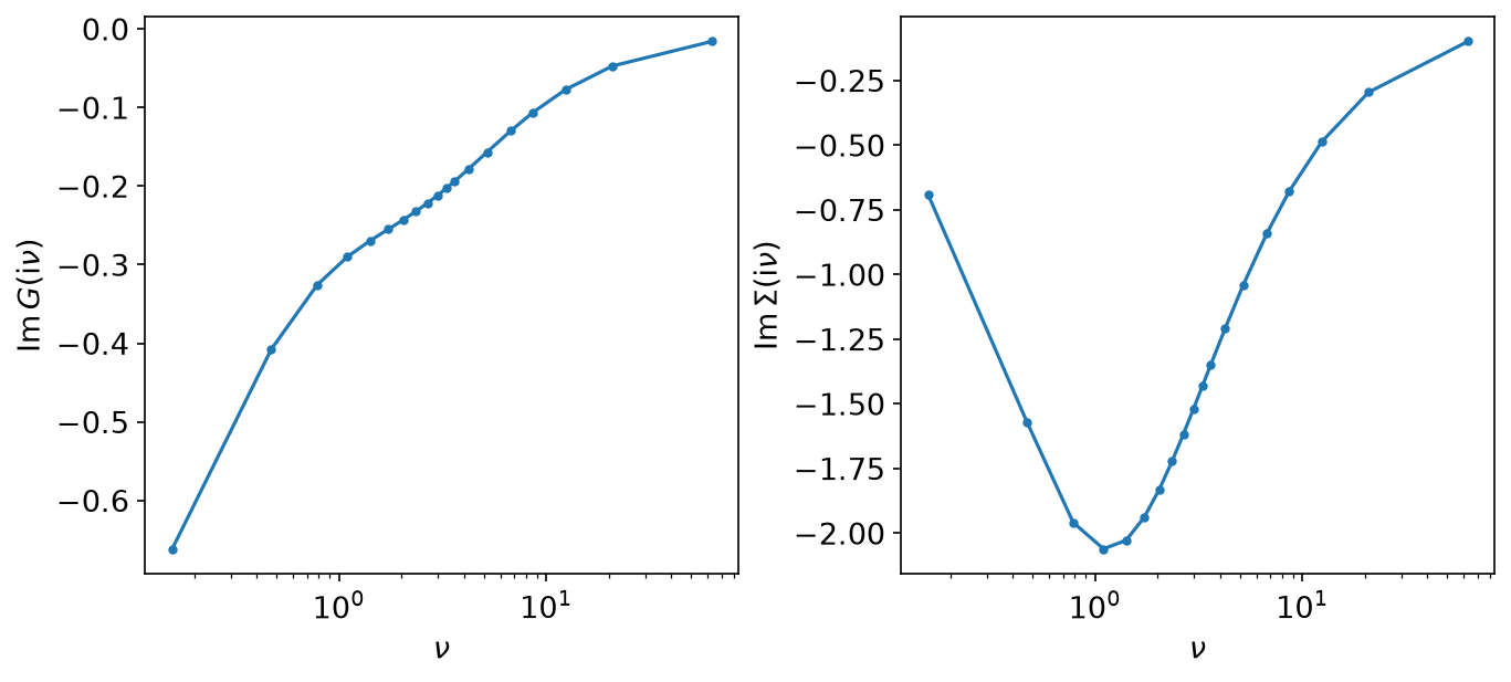
Left to run for 5000 iterations, the same loop settles on the same metal: the residual reaches \(10^{-16}\) by iteration 270 and stays there, and \(Z = 0.26307\) differs from the stopped run’s \(0.26310\) in the fifth digit, about what a threshold of \(10^{-5}\) on the change promises.
Now switch the projection off. Nothing else changes — same start, same mixing — and the run follows the symmetric one for 60 iterations, then leaves it:
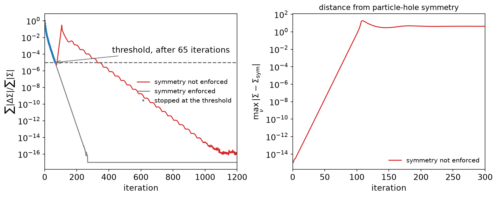
The right panel is the reason. The distance of \(\Sigma\) from its symmetric part starts at the \(10^{-15}\) of rounding and grows by about 40% per iteration, a straight line on the log scale, until it is of order one after 100 iterations. The symmetric metal is a fixed point of the loop, but an unstable one with respect to perturbations that break the symmetry, and rounding supplies such a perturbation at every step. The unprojected run then converges again (left panel, red) — to a state whose self-energy is far from particle-hole symmetric, which the exact solution of this half-filled model cannot be. Which broken state it reaches, and when it leaves, depends on the last bits of the arithmetic: two implementations, or two BLAS backends, generally land on different ones.
The moral is not specific to IR. A self-consistency loop converges to the fixed points that are stable under its own iteration, which need not be the physical ones; if the physical solution has a symmetry, impose it.
Scanning \(U\): the Mott transition and its hysteresis
dmft_ipt_scan sweeps \(U\) from 0 to 6.5 in 66 steps, three times:
- starting each \(U\) from the non-interacting \(G^0\);
- sweeping upwards, starting each \(U\) from the previous solution (the metal branch);
- sweeping downwards from \(U = 6.5\) (the insulator branch).
Every solve runs a fixed 5000 iterations with no stopping rule, so every point is a fixed point to machine precision rather than a snapshot on the way to one; the slowest, next to the edges of the coexistence window, are converged long before that.
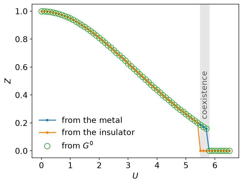
\(Z\) falls smoothly from 1 and then drops to zero, but not at the same \(U\) going up as coming down. The metal exists up to \(U = 5.7\) and is gone at 5.8, so \(U_{c2}\) lies between the two. Walking down, the insulator survives to \(U = 5.5\). In between both solutions are stable and which one you get depends on where you started: that shaded window is the first-order Mott transition. Its lower edge depends on how it is approached — started directly from the \(U = 6.5\) insulator instead of from its neighbour, the loop still finds an insulator at \(U = 5.3\) — which is the usual caveat about mapping a coexistence region with a simple iteration.
Starting from \(G^0\) lands on the metal branch wherever the metal exists —
the from_g0 and metal columns agree to \(10^{-15}\) across the whole
grid — which is why a naive scan sees only \(U_{c2}\) and misses the
hysteresis entirely.
The self-energies on either side make the distinction concrete:
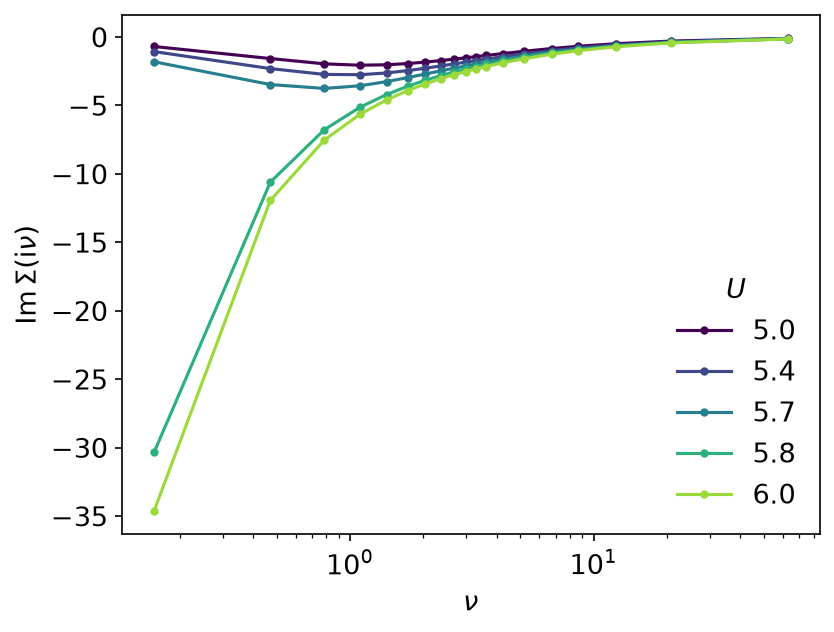
These are the solves started from \(G^0\), so they are on the metal branch wherever it exists. At \(U = 5.0, 5.4, 5.7\) \(\mathrm{Im},\Sigma\) turns back towards zero at the lowest frequencies, a Fermi liquid with a strongly reduced \(Z\). At \(U = 5.8\) and \(U = 6.0\) it diverges as \(\nu \to 0\), which is the pole at the Fermi level that opens the Mott gap.
Without the projection, this scan finds a “transition” between \(U = 3.4\) and \(3.5\) instead: there the symmetry-breaking instability of the previous section sets in within 5000 iterations, and the loop leaves the metal for a broken-symmetry state long before the metal ceases to exist.
Beyond the imaginary axis
Everything above lives on the imaginary axis. The contrast between the metal and the Mott insulator is most visible in the spectral function \(A(\omega)\) — a quasiparticle peak at \(\omega = 0\) against a gap between two Hubbard bands — and getting there from \(G(\mathrm{i}\nu)\) is analytic continuation. The IR coefficients \(g_l\) computed here are the natural input: see analytic continuation for regularised inversion of \(g_l = -s_l\rho_l\), sparse modeling for the \(\ell_1\)-regularised version, and MiniPole for a pole representation of \(G(\mathrm{i}\nu)\) from which \(A(\omega)\) can be read off.
Running it
From docs/tutorial-code:
$ cargo run --profile ci --bin dmft_ipt
$ cargo run --profile ci --bin dmft_ipt_scan
$ uv run --project ../plotting python ../plotting/dmft_ipt_plot.py
dmft_ipt takes about a second. dmft_ipt_scan is 198 self-consistent
solves of 5000 iterations each, which is closer to half a minute. The
binaries write CSV tables under docs/tutorial-code/data/; the plotting
script only reads them.
The repository checks these numbers against a Python version of the notebook’s loop with the same symmetry projection. The run without the projection is compared only by its shape, since where it ends up is decided by rounding.
Key API pieces
From sparse-ir:
| What you want | What to call |
|---|---|
| the fermionic IR basis at \(\beta\), \(\omega_\mathrm{max}\), \(\varepsilon\) | LogisticKernel::new, FiniteTempBasis::<_, Fermionic>::new |
| sampling in \(\tau\) and \(\mathrm{i}\nu\) | TauSampling::new, MatsubaraSampling::new (wrapped by IrMesh) |
| \(s_l\) and \(v_l(\omega)\) for \(g_l = -s_l\rho_l\) | basis.s(), basis.v() (get_knots, get_polyorder) |
| the reduced index of a sampling frequency | MatsubaraFreq::n |
From the tutorial crate (docs/tutorial-code/src):
| What you want | Tutorial helper |
|---|---|
| \(\tau \to \mathrm{i}\nu\) and back, once per iteration | IrMesh::tau_to_wn, IrMesh::wn_to_tau |
| \(\rho_l\) of a semicircle, by quadrature | shifted_semicircle_overlaps, then IrMesh::l_to_wn |
| \(\Sigma(\tau)\) for plotting | IrMesh::wn_to_l, then IrMesh::l_to_tau |
| the lowest Matsubara frequency | the position of \(n = 1\) in IrMesh::wn |
Two-particle self-consistency
Ported from the Python notebook
TPSC_py.ipynb
of the sparse-ir tutorials,
whose author is Niklas Witt. The programs that produced every number and
figure on this page are docs/tutorial-code/src/bin/tpsc.rs and
docs/tutorial-code/src/bin/tpsc_scan.rs; the solver is in
docs/tutorial-code/src/tpsc.rs, and the code below is included from there.
The previous page iterated a self-consistency loop thousands of times. This one does not iterate at all: the two-particle self-consistent approach fixes its vertices by solving two scalar equations, and the whole calculation is a single pass through the basis with a pair of root searches in the middle.
Vertices from sum rules
TPSC starts where RPA starts, with the irreducible susceptibility of the square lattice at half bandwidth \(4t\),
\[ \chi^0(\mathrm{i}\omega, q) ;=; -\frac{1}{N_k}\sum_{k} \int_0^\beta \mathrm{d}\tau; \mathrm{e}^{\mathrm{i}\omega\tau}, G(\tau, k), G(-\tau, k - q), \]
with \(\mathrm{i}\omega\) a bosonic Matsubara frequency (even reduced index) and \(\mathrm{i}\nu\) a fermionic one (odd), as in the conventions, and dresses it in the usual geometric way,
\[ \chi_\mathrm{sp} = \frac{\chi^0}{1 - U_\mathrm{sp}\chi^0}, \qquad \chi_\mathrm{ch} = \frac{\chi^0}{1 + U_\mathrm{ch}\chi^0}. \]
What is different is where \(U_\mathrm{sp}\) and \(U_\mathrm{ch}\) come from. RPA sets both to the bare \(U\) and is done. TPSC instead demands that the two susceptibilities satisfy the local sum rules exactly,
\[ \frac{2}{N_k\beta}\sum_{q,\omega} \chi_\mathrm{sp}(\mathrm{i}\omega, q) = n - 2\langle n_\uparrow n_\downarrow\rangle, \qquad \frac{2}{N_k\beta}\sum_{q,\omega} \chi_\mathrm{ch}(\mathrm{i}\omega, q) = n + 2\langle n_\uparrow n_\downarrow\rangle - n^2, \]
where \(n\) on the right is the filling, and closes the first of them with the Kanamori–Brueckner ansatz \(\langle n_\uparrow n_\downarrow\rangle = \tfrac14 (U_\mathrm{sp}/U),n^2\). That makes the spin rule an equation in \(U_\mathrm{sp}\) alone; the double occupancy that comes out of it then makes the charge rule an equation in \(U_\mathrm{ch}\) alone. Two one-dimensional root searches, no loop.
The sums on the left are the reason this page belongs in a basis tutorial. A sum over every bosonic Matsubara frequency is, in the basis, the value of the zone-averaged susceptibility at \(\tau = 0\): fit once, evaluate once.
    let chi = rpa(chi_0, vertex);
    let averaged: Vec<Complex64> = (0..lattice.mesh_b().n_wn())
        .map(|i| chi[i * nk..(i + 1) * nk].iter().sum::<Complex64>() / nk as f64)
        .collect();
    let coefficients = lattice.mesh_b().wn_to_l(&averaged, 1)?;
    Ok(evaluate_rows(lattice.ub_at_zero(), &coefficients, 1)[0].re)
Each evaluation of the sum rule costs one fit of 31 sampling points onto 30 basis functions and one evaluation of \(u^B_l(0)\), so putting it inside a root search (Brent’s method) is affordable. With a truncated Matsubara sum it would not be: the tail of \(\chi\) decays as \(1/\omega^2\) and the sum rule is precisely the quantity that tail controls.
\(\chi^0\) itself is the same convolution as on the GW page, built as a product in \((\tau, r)\):
    let grt = {
        let gkt = lattice.mesh_f().wn_to_tau(gkio, nk)?;
        lattice.grid().k_to_r(&gkt)
    };
    let reversed = lattice.mesh_f().reverse_tau(&grt, nk);
    let product: Vec<Complex64> = grt.iter().zip(&reversed).map(|(a, b)| a * b).collect();
    let in_momentum = lattice.grid().r_to_k(&product);
    lattice.mesh_b().tau_to_wn(&in_momentum, nk)
The one subtlety is reverse_tau. It returns \(G(\beta - \tau)\): the
sampling points read backwards together with the fermionic sign,
\(G(\beta - \tau) = -G(-\tau)\). The product is therefore
\(-G(\tau)G(-\tau)\), which is where the minus sign in \(\chi^0\) comes
from. Reading the points backwards works because the sampling times lie on
\([-\beta/2, \beta/2]\) and are (nearly) symmetric about \(0\) — a
point at \(\beta/2\) is matched with its image one period away;
tau_reversal panics if some \(-\tau\) is missing. And the fermionic and
bosonic \(\tau\) grids coincide, because the logistic kernel gives both
statistics the same \(u_l(\tau)\); Bases::from_sve asserts that the two
grids are equal. That is what lets the product, sampled on fermionic times,
be fitted with the bosonic sampling object.
With the two vertices fixed, the self-energy is one more product in \((\tau, r)\),
\[ \Sigma(\tau, r) = V(\tau, r), G(\tau, r), \qquad V = \frac{U}{4}\left(3U_\mathrm{sp}\chi_\mathrm{sp} + U_\mathrm{ch}\chi_\mathrm{ch}\right), \]
built from the non-interacting \(G\), after which \(\mu\) is refixed for the interacting \(G\). As on the FLEX page, the instantaneous Hartree shift is left out of \(V\) and absorbed into \(\mu\).
One solve at U = 4
tpsc takes a \(24 \times 24\) lattice at \(\beta = 10\), filling
\(n = 0.85\), \(U = 4\) and \(\varepsilon = 10^{-10}\). The basis has 30
functions for each statistics, giving 30 \(\tau\) points, 30 fermionic and
31 bosonic frequencies — the entire frequency content of a lattice problem at
\(\beta\omega_\mathrm{max} = 100\).
The vertices come out as
\[ U_\mathrm{sp} = 2.1011 ;<; U = 4 ;<; U_\mathrm{ch} = 7.6738, \]
which is the qualitative statement TPSC exists to make: spin fluctuations screen the interaction in the spin channel and anti-screen it in the charge channel, and RPA’s \(U_\mathrm{sp} = U\) overshoots badly. The double occupancy is \(0.0949\), well below the uncorrelated \((n/2)^2 = 0.1806\).
Note also \(U_\mathrm{crit} = 1/\max\chi^0 = 2.3821\). The spin sum rule has
no solution above it — the RPA denominator would change sign — so
\(U_\mathrm{sp}\) is bounded by \(U_\mathrm{crit}\) no matter how large
\(U\) grows. That bound is what enforces the Mermin–Wagner theorem here, and
a request that would violate it is reported as TpscError::Ordered rather
than producing a number.
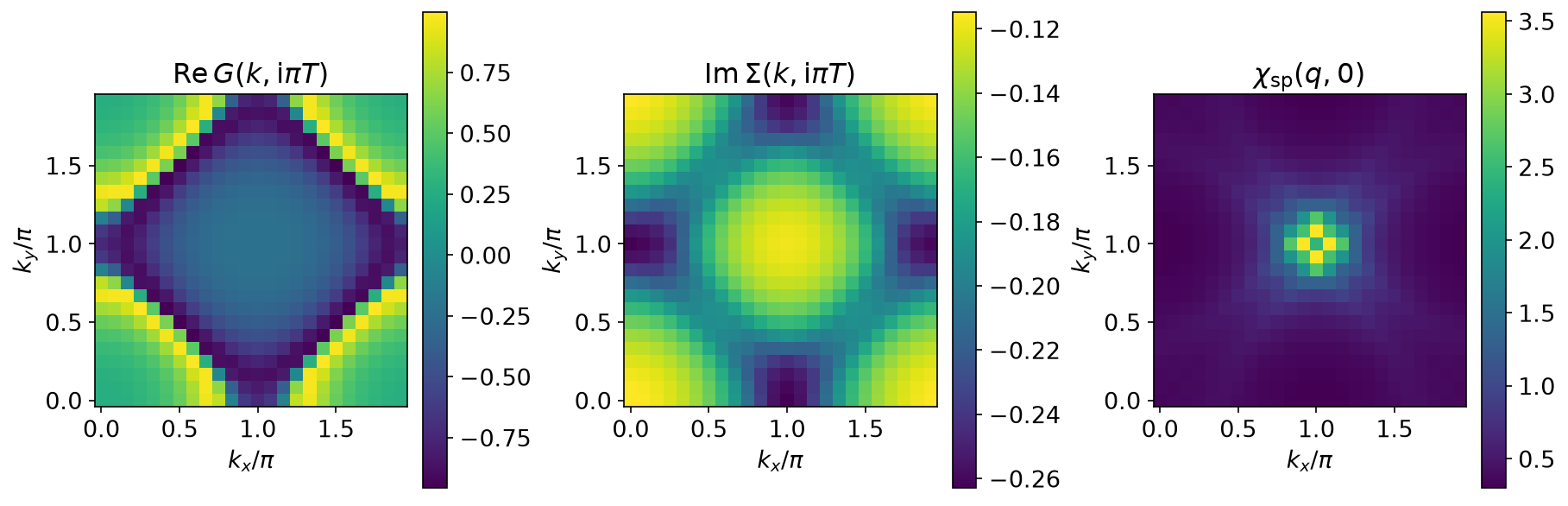
The zeroth Matsubara slice shows a Fermi surface in \(\mathrm{Re},G\), \(|\mathrm{Im},\Sigma|\) largest near the antinodes \((\pi, 0)\) — the beginning of the pseudogap — and \(\chi_\mathrm{sp}\) piled up around \(M = (\pi,\pi)\).
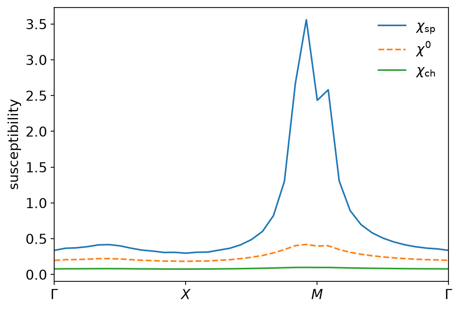
Along the high-symmetry path the ordering \(\chi_\mathrm{sp} > \chi^0 > \chi_\mathrm{ch}\) holds everywhere, and the enhancement is strongly momentum-selective: a factor of about 8.5 at the peak against 1.7 at \(\Gamma\). The peak is not at \(M\). At \(n = 0.85\) the system is doped, nesting is incommensurate, and the maximum sits one grid step away at \((\pi, 11\pi/12)\) with the value \(3.559\) against \(2.434\) at \(M\) itself.
Scanning U
tpsc_scan repeats the solve at half filling and \(T = 0.4\) for 51 values
of \(U\) from \(0.01\) to \(5\), which is the sweep behind Fig. 2 of
Y. M. Vilk and A.-M. S. Tremblay, J. Phys. I France 7, 1309 (1997).
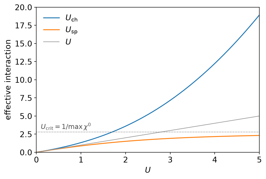
\(U_\mathrm{crit} = 2.7789\) is a property of \(\chi^0\), which does not depend on \(U\), and so is the same at every point of the scan. \(U_\mathrm{sp}\) rises from \(0.00999\) and flattens against that ceiling, reaching \(2.318\), i.e. \(83%\) of \(U_\mathrm{crit}\), at \(U = 5\). \(U_\mathrm{ch}\) has no such bound and runs away to \(18.9\). Between them the double occupancy falls from \(0.2497\) — the uncorrelated \(1/4\) — to \(0.1159\).
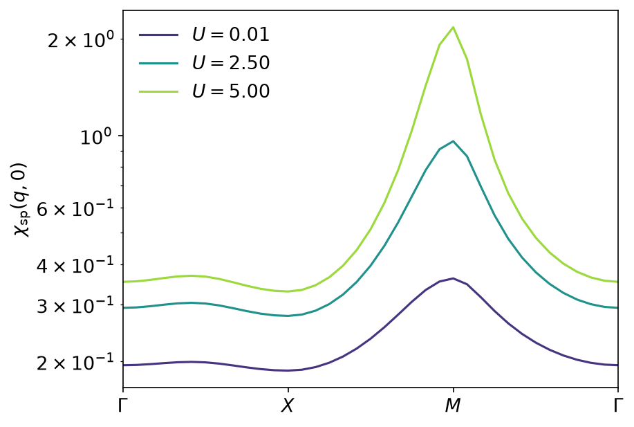
The susceptibility at half filling does peak at \(M\), and it grows by a factor of six there between \(U = 0.01\) and \(U = 5\) while barely doubling at \(\Gamma\). The saturating \(U_\mathrm{sp}\) is what keeps that growth finite: in RPA the same sweep would have diverged long before \(U = 5\).
Beyond the imaginary axis
The output here is \(G\), \(\Sigma\) and \(\chi\) on the sampling frequencies. For real-frequency spectra — the pseudogap in \(A(k,\omega)\), say — see analytic continuation, sparse modeling and MiniPole; for a compact pole representation of the same data, see the DLR.
Running it
From docs/tutorial-code:
$ cargo run --profile ci --bin tpsc
$ cargo run --profile ci --bin tpsc_scan
$ uv run --project ../plotting python ../plotting/tpsc_plot.py
Both programs are fast. tpsc is a single solve of a \(24\times24\)
lattice; tpsc_scan is 51 of them at a smaller basis and finishes in a
fraction of a second. The repository’s checks compare the outputs with the
Python notebook; they also assert that the \(n = 0.85\) peak lies on
\(k_x = \pi\) within one grid step of \(M\) (not at \(M\)) and that
\(U_\mathrm{crit}\) is constant along the scan.
Key API pieces
From sparse-ir:
| What you want | What to call |
|---|---|
| one SVE for both statistics | compute_sve, then FiniteTempBasis::from_sve_result twice |
| \(u_l(0)\), the row that turns a Matsubara sum into an evaluation | Basis::evaluate_tau(&[0.0]) |
| fits and evaluations at the sampling points | TauSampling, MatsubaraSampling (wrapped by IrMesh) |
From the tutorial crate (docs/tutorial-code/src):
| What you want | Tutorial helper |
|---|---|
| a Matsubara sum over all frequencies | IrMesh::wn_to_l, then evaluate_rows with \(u^B_l(0)\) |
| \(G(\beta - \tau) = -G(-\tau)\) on the sampling grid | IrMesh::reverse_tau |
| a fermionic product fitted as bosonic | IrMesh::wn_to_tau on one mesh, IrMesh::tau_to_wn on the other |
| both bases and meshes from one SVE | sve_for, Bases::from_sve (inside Lattice::new) |
| \(\chi^0\) as a real-space product | MomentumGrid::k_to_r, MomentumGrid::r_to_k |
| solving a sum rule for a vertex | brent from tutorial::roots |
Fluctuation exchange
Ported from the Python notebook
FLEX_py.ipynb
of the sparse-ir tutorials,
whose author is Niklas Witt. The programs that produced every number and
figure on this page are docs/tutorial-code/src/bin/flex.rs and
docs/tutorial-code/src/bin/flex_scan.rs; the solver is in
docs/tutorial-code/src/flex.rs, and the code below is included from there.
The previous page fixed its vertices by solving two scalar equations and never iterated. The fluctuation-exchange approximation goes the other way: the interaction stays the bare \(U\), and everything is decided by a Dyson loop that is run until the self-energy stops moving. What makes it belong here is that each pass of that loop is a handful of products in \((\tau, r)\) with basis transforms between them — the frequency dependence never appears as a truncated sum.
One loop, four transforms
FLEX sums the particle-hole bubble and ladder series, which in a single band collapses to a self-energy built from the same irreducible \(\chi^0\) as on the TPSC page, dressed twice:
\[ \chi_\mathrm{sp} = \frac{\chi^0}{1 - U\chi^0}, \qquad \chi_\mathrm{ch} = \frac{\chi^0}{1 + U\chi^0}, \qquad V = U^2\left(\tfrac32 \chi_\mathrm{sp} + \tfrac12 \chi_\mathrm{ch} - \chi^0\right), \]
\[ \Sigma(\tau, r) = V(\tau, r), G(\tau, r), \qquad G(\mathrm{i}\nu, k) = \bigl[\mathrm{i}\nu - (\varepsilon_k - \mu) - \Sigma(\mathrm{i}\nu, k)\bigr]^{-1}. \]
Here \(\mathrm{i}\omega\) is a bosonic and \(\mathrm{i}\nu\) a fermionic Matsubara frequency, as in the conventions. Read as code, one step is: dress \(\chi^0\) in \((\mathrm{i}\omega, q)\), carry \(V\) to \((\tau, r)\), multiply by \(G(\tau, r)\), carry the product back to \((\mathrm{i}\nu, k)\).
        let v: Vec<Complex64> = (0..self.ckio.len())
            .map(|i| u * u * (1.5 * self.chi_spin[i] + 0.5 * self.chi_charge[i] - self.ckio[i]))
            .collect();
        let in_real_space = self.lattice.grid().k_to_r(&v);
        Ok(self.lattice.mesh_b().wn_to_tau(&in_real_space, nk)?)

        let product: Vec<Complex64> = interaction
            .iter()
            .zip(&self.grit)
            .map(|(v, g)| v * g)
            .collect();
        let in_momentum = self.lattice.grid().r_to_k(&product);
        Ok(self.lattice.mesh_f().tau_to_wn(&in_momentum, nk)?)
The bosonic mesh fits the interaction and the fermionic one fits the self-energy, on the same \(\tau\) grid — the point the TPSC page already relied on. The two grids coincide because the logistic kernel gives both statistics the same \(u_l(\tau)\); sharing one SVE between them only saves the second expansion.
Written in full, \(V\) would also carry the first-order term, a bare instantaneous \(U\) (a \(\delta(\tau)\) term). It is left out: it is frequency independent, so the basis is the wrong tool for it, and in \(\Sigma\) it would be the Hartree shift \(Un/2\), which in a single band is a shift of the chemical potential, refitted at every step anyway. That omission comes back in the gap equation below.
Keeping the denominator positive
Nothing forces \(1 - U\chi^0\) to stay positive along the way to the fixed point, and \(\chi^0\) evaluated on the non-interacting Green’s function is the largest it will ever be. At \(U = 4\) the starting point does violate it, so the interaction is walked up instead of being switched on at once:
        while target * self.max_chi() >= 1.0 {
            self.renormalisation_steps += 1;
            self.u = target / (self.max_chi() * target + 0.01);
            self.step()?;
            self.u = target;
            if self.renormalisation_steps == self.settings.renormalisation_iterations {
                break;
            }
        }
Each pass runs one FLEX step at the largest interaction the current
\(\chi^0\) can carry, which shrinks \(\chi^0\); the target \(U\) is then
retried. The loop is capped, because there is no guarantee it ever succeeds:
a genuinely ordered system has no FLEX solution to walk towards. At
\(T = 0.1\) six passes are enough; the number is written out as
renormalisation_steps.
One solve at U = 4
flex takes a \(24 \times 24\) lattice at \(\beta = 10\), filling
\(n = 0.85\), \(U = 4\), \(\varepsilon = 10^{-10}\) and a linear mixing
of \(0.2\), and runs 30 steps. The basis has 30 functions for each
statistics: 30 \(\tau\) points, 30 fermionic and 31 bosonic frequencies. The
relative movement of \(\Sigma\) in the last step is \(1.3\times10^{-5}\),
and \(\mu = -0.6713\).
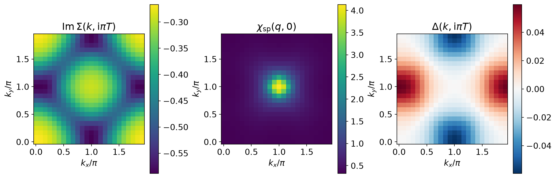
\(|\mathrm{Im},\Sigma|\) is largest at the antinodes \((\pi, 0)\) and smallest along the diagonal — the momentum-selective scattering that opens a pseudogap — and \(\chi_\mathrm{sp}\) is piled up at \(M = (\pi, \pi)\), enhanced there by a factor of \(17.5\) over \(\chi^0\) against \(2.3\) at \(\Gamma\).
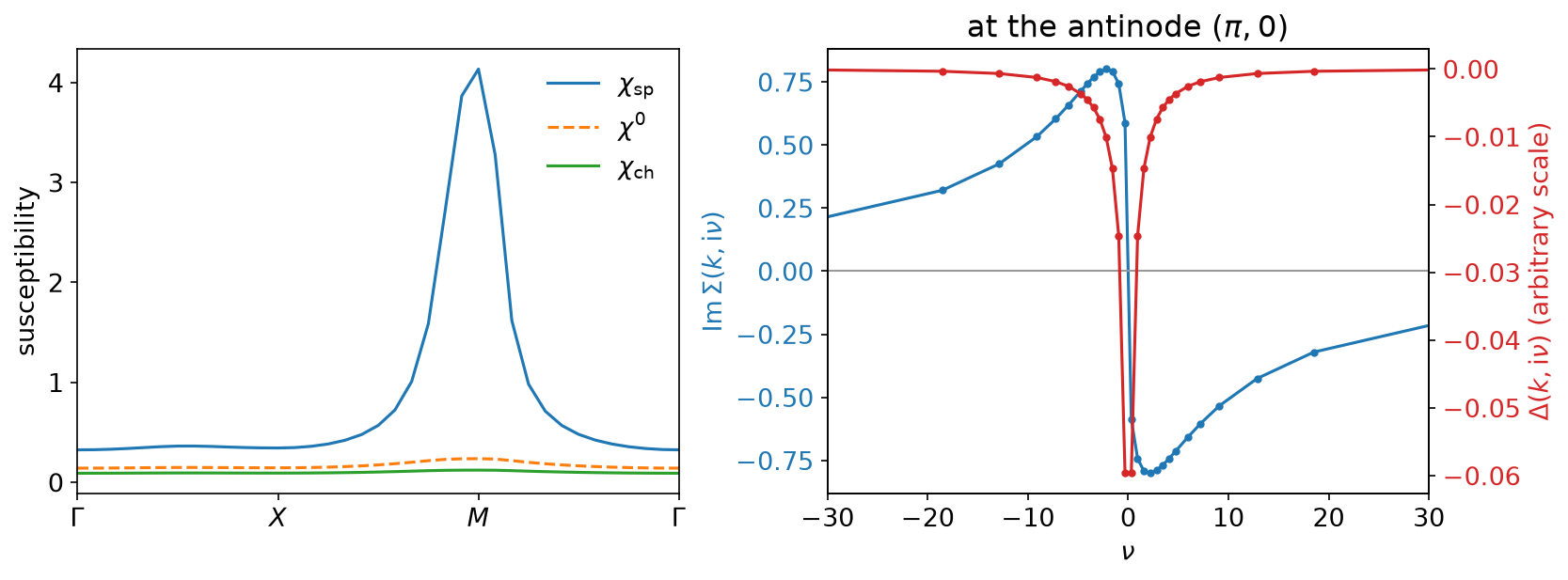
Against frequency, \(\mathrm{Im},\Sigma\) is odd, largest in magnitude at the first Matsubara frequency and decaying from there; the run gives \(\mathrm{Im},\Sigma(\mathrm{i}\pi T, (\pi,0)) = -0.588\). Its sign, opposite to that of \(\nu\) at every sampling frequency, is the statement that the solution is causal.
The linearised gap equation
With the fluctuations in hand, the question is whether they pair. The linearised Eliashberg equation
\[ \lambda, \Delta(\mathrm{i}\nu, k) = \frac{T}{N_k} \sum_{\mathrm{i}\nu’, k’} V^S(\mathrm{i}\nu - \mathrm{i}\nu’, k - k’), F(\mathrm{i}\nu’, k’), \qquad F = -|G|^2,\Delta, \]
is an eigenvalue problem whose leading \(\lambda\) reaches 1 at \(T_\mathrm{c}\). (The sign is carried by \(F\), as in the code; writing \(F = |G|^2\Delta\) with a minus sign in front of the sum is the same equation.) The convolution is a plain product \(V^S(\tau, r)F(\tau, r)\). The singlet vertex is not the one in the self-energy: the charge fluctuations enter with the opposite sign, \(V^S = U + U^2\left(\tfrac32\chi_\mathrm{sp} - \tfrac12\chi_\mathrm{ch}\right)\), of which the code keeps the frequency-dependent part. Applying it is the same four transforms as one FLEX step, so the power method costs about what a few self-consistency steps cost, seeded with a \(d_{x^2-y^2}\) gap \(\cos k_x - \cos k_y\).
Here the dropped bare \(U\) (the \(\delta(\tau)\) term of \(V^S\)) matters. It contributes exactly zero in the \(d\)-wave channel, because such a gap sums to zero over the zone, but not outside it, and without it the operator has a spurious mode whose eigenvalue is \(-1.28\) — larger in magnitude than \(\lambda_d\). The seed has almost no overlap with it, so the iterate sits on the \(d\)-wave answer for tens of steps and then leaves it. A fixed step count would land right at that crossover; the loop therefore stops when \(\lambda\) moves by less than \(10^{-4}\), which happens after 8 steps with three orders of magnitude to spare. The step count is written out too.
The result is \(\lambda_d = 0.4568\) at \(T = 0.1\): the right symmetry, well short of the transition. The gap in the third panel above changes sign under \(k_x \leftrightarrow k_y\) and vanishes on the zone diagonal; the eigenvector’s overall scale means nothing, only its shape does.
(The \(\lambda\) here is an eigenvalue of the gap equation. It is unrelated to the electron-phonon coupling \(\lambda_0\) of the Eliashberg page.)
Cooling towards T_c
flex_scan repeats the calculation on a \(64 \times 64\) lattice at seven
temperatures from \(T = 0.08\) down to \(0.025\), with
\(\Lambda = \beta\omega_\mathrm{max}\) held at \(10^3\) and
\(\varepsilon = 10^{-8}\). Holding \(\Lambda\) fixed means one SVE serves
every temperature —
    let beta_init = 1.0 / TEMPERATURES[0];
    let (kernel, sve) = sve_for(beta_init, LAMBDA / beta_init, EPS)?;
// ...
    for (index, &temperature) in TEMPERATURES.iter().enumerate() {
        let beta = 1.0 / temperature;
        let lattice = Lattice::from_sve(kernel, sve.clone(), NK_LIN, NK_LIN, T_HOP, beta, EPS)?;
— and that every temperature has a basis of the same 43 functions, which in turn is what makes it legal to carry the converged \(\Sigma\) of one temperature into the next as a starting point. With that head start, the renormalisation loop runs only at the first temperature (nine passes) and never again.
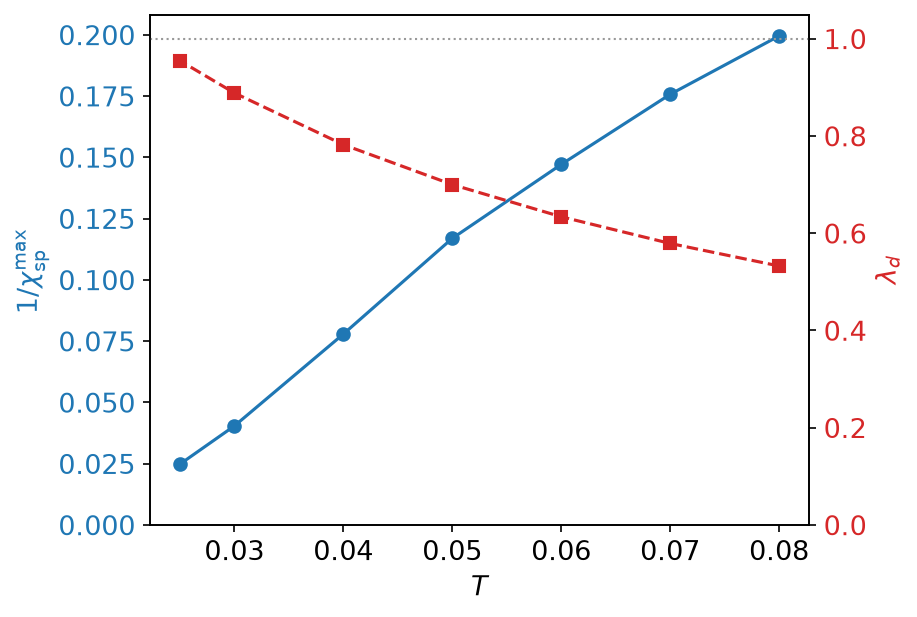
\(1/\chi_\mathrm{sp}^{\max}\) falls almost linearly — the Curie–Weiss form — from \(0.1996\) to \(0.0248\), extrapolating to zero near \(T \approx 0.019\), while \(\lambda_d\) climbs from \(0.533\) to \(0.955\) and would reach 1 at about \(T \approx 0.021\). The two temperatures are close because in this approximation it is the spin fluctuations that do the pairing: the gap equation is driven by the same \(\chi_\mathrm{sp}\) that is diverging.
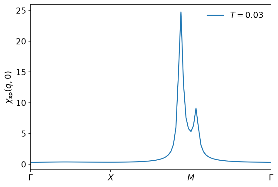
The finer grid also resolves what the \(24\times24\) run could not: at \(n = 0.85\) the peak is not at \(M\). Nesting is incommensurate, and \(\chi_\mathrm{sp}\) peaks at \((\pi, 7\pi/8)\) with the value \(24.8\) against \(5.3\) at \(M\) itself — a factor of nearly five that a commensurate grid would have missed entirely.
Beyond the imaginary axis
FLEX gives \(\Sigma\), \(\chi\) and \(\Delta\) on the sampling frequencies only. To look at the pseudogap or the gap on the real axis, the same data have to be continued: see analytic continuation, sparse modeling and MiniPole. The DLR gives a pole representation of the same functions on the imaginary axis.
Running it
From docs/tutorial-code:
$ cargo run --profile ci --bin flex
$ cargo run --profile ci --bin flex_scan
$ uv run --project ../plotting python ../plotting/flex_plot.py
flex is one solve and takes under half a second; flex_scan is seven solves
on a grid seven times larger and takes a few seconds. The repository’s checks
compare the outputs with the Python notebook, including the
renormalisation-pass and power-method step counts, the sign of
\(\mathrm{Im},\Sigma\) at every frequency, and the symmetry of the gap.
Key API pieces
From sparse-ir:
| What you want | What to call |
|---|---|
| one SVE reused across temperatures | compute_sve with LogisticKernel::new(Λ), then FiniteTempBasis::from_sve_result per \(\beta\) |
| \(u^F_l(0^+)\) for the filling | Basis::evaluate_tau(&[0.0]) (\(+0.0\) means \(0^+\)) |
| fits and evaluations at the sampling points | TauSampling, MatsubaraSampling (wrapped by IrMesh) |
From the tutorial crate (docs/tutorial-code/src):
| What you want | Tutorial helper |
|---|---|
| one step of a Dyson loop | IrMesh::wn_to_tau, MomentumGrid::k_to_r, multiply, MomentumGrid::r_to_k, IrMesh::tau_to_wn |
| \(\chi^0\) as a real-space product | IrMesh::reverse_tau, then the bosonic IrMesh::tau_to_wn |
| the filling \(n = 2[1 + G(\tau = 0^+)]\) | IrMesh::wn_to_l, then evaluate_rows with \(u^F_l(0^+)\) |
| the chemical potential at fixed \(n\) | brent from tutorial::roots |
| one SVE reused across temperatures | sve_for, then Lattice::from_sve per \(\beta\) |
| a whole basis at fixed \(\Lambda\) | keep \(\beta\omega_\mathrm{max}\) constant and vary \(\beta\) |
Eliashberg theory
Ported from the Python notebook
eliashberg_holstein_py.ipynb
of the sparse-ir tutorials,
whose authors are Shintaro Hoshino and Hiroshi Shinaoka. The programs that
produced every number and figure on this page are
docs/tutorial-code/src/bin/eliashberg_holstein.rs and
docs/tutorial-code/src/bin/eliashberg_holstein_scan.rs; the solver is in
docs/tutorial-code/src/eliashberg.rs, and the code below is included from
there.
The lattice examples before this one carried a momentum index; this one, like the DMFT page, does not. The electrons have a semicircular density of states of half bandwidth \(D = 0.5\), \(\rho(\omega) = \tfrac{2}{\pi D^2}\sqrt{D^2 - \omega^2}\), and couple to local phonons of frequency \(\omega_0 = 0.15\). Every self-energy is local, so the momentum dependence collapses into a single quadrature over \(\omega\). What is left is the smallest self-consistent calculation the basis is useful for, and the one where its compactness is easiest to see: at \(\beta = 500\) the whole solution — four functions of frequency — lives in 45 basis functions.
The model
Despite the file name, the model solved here is not the single-band Holstein model but its three-orbital generalisation, the Jahn–Teller–Hubbard model relevant to the fulleride superconductors (Y. Kaga, P. Werner and S. Hoshino, Phys. Rev. B 105, 214516 (2022)): three degenerate orbitals with a Hubbard \(U = 2\) and a Hund’s coupling \(J = 0.03,U = 0.06\), coupled to six local phonon modes of the same frequency \(\omega_0\) and the same coupling \(g_0\). The coupling is set by the dimensionless electron-phonon coupling \(\lambda_0\) through
\[ g_0 = \sqrt{\tfrac34,\lambda_0,\omega_0}, \]
with \(\lambda_0 = 0.125\) for the single solve below and \(\lambda_0 = 0.175\) for the temperature scan. With cubic symmetry and a local self-energy, all three orbitals carry the same \(G\), \(F\), \(\Sigma\) and \(\Delta\), and the multi-orbital structure survives only in prefactors: the effective interaction is
\[ U_\mathrm{eff}(\tau) = (U + 2J),\delta(\tau) + (M + 1),g_0^2,\mathcal{D}(\tau), \qquad M = 3, \]
which is where the \(4g_0^2\) below comes from, and the internal energy carries an overall factor \(3\) (\(M = 3\)). With \(M = 1\) and \(J = 0\) the same equations describe the single-orbital Holstein–Hubbard model.
On notation: \(D\) is the half bandwidth (the program’s D), and
\(\mathcal{D}\) the phonon propagator (d_iv, d_tau). The coupling
\(\lambda_0\) is an input parameter; it has nothing to do with the
eigenvalue \(\lambda\) of the FLEX gap equation.
The equations
The electrons are described by the normal \(G\) and the anomalous \(F\), which in the superconducting state are both non-zero:
\[ G(\mathrm{i}\nu) = \int\!\mathrm{d}\omega\,\rho(\omega)\, \frac{\xi(\mathrm{i}\nu) + \omega} {\xi(\mathrm{i}\nu)^2 - \Delta(\mathrm{i}\nu)^2 - \omega^2}, \qquad F(\mathrm{i}\nu) = \int\!\mathrm{d}\omega\,\rho(\omega)\, \frac{\Delta(\mathrm{i}\nu)} {\xi(\mathrm{i}\nu)^2 - \Delta(\mathrm{i}\nu)^2 - \omega^2}, \]
with \(\xi = \mathrm{i}\nu + \mu - \Sigma\) and \(\mu = 0\) (half filling). The phonon is dressed by the electrons it couples to, and dresses them back (\(\mathrm{i}\omega\) is a bosonic frequency):
\[ \Pi(\tau) = -4g_0^2\left[G(\tau)G(\beta - \tau) + F(\tau)^2\right], \qquad \mathcal{D}(\mathrm{i}\omega) = \left[\mathcal{D}_0(\mathrm{i}\omega)^{-1}
- \Pi(\mathrm{i}\omega)\right]^{-1}, \qquad \mathcal{D}_0(\mathrm{i}\omega) = \frac{2\omega_0}{(\mathrm{i}\omega)^2 - \omega_0^2}, \] \[ \Sigma(\tau) = -4g_0^2\,\mathcal{D}(\tau)G(\tau), \qquad \Delta(\tau) = 4g_0^2\,\mathcal{D}(\tau)F(\tau) + (U + 2J)\,F(\tau_0)\delta(\tau). \]
The instantaneous \((U + 2J)F\) term is the Coulomb repulsion, which fights the phonon; the rest is retarded, and it is that retardation that lets superconductivity survive a bare repulsion of \(U = 2\) against a phonon of \(\omega_0 = 0.15\). Strictly the instantaneous term needs \(F(0^+)\); the program, like the notebook, reads \(F\) at the smallest positive sampling time \(\tau_0\) instead. That is an approximation to the limit, not the limit itself.
One pass of the loop is therefore a handful of transforms and products — \(G\) and \(F\) to \(\tau\), then the phonon, then the electron self-energies (the particle-hole symmetrisation and the clip discussed below sit between the first two steps):
            let (g_iv, f_iv) = self.green();
            self.g_iv = g_iv;
            self.f_iv = f_iv;
            let mut g_tau = mesh_f.wn_to_tau(&self.g_iv, 1)?;
            let f_tau = mesh_f.wn_to_tau(&self.f_iv, 1)?;
            // `Π(τ) = −4g² [G(τ)G(β − τ) + F(τ)²]`, fitted as a bosonic
            // function of the shared τ grid.
            let reversed = mesh_f.reverse_tau(&g_tau, 1);
            let phi_tau: Vec<Complex64> = (0..g_tau.len())
                .map(|i| -four_g2 * (g_tau[i] * reversed[i] + f_tau[i] * f_tau[i]))
                .collect();
            self.phi_iv = mesh_b.tau_to_wn(&phi_tau, 1)?;
            // `Π` is real by construction; what the transforms leave in the
            // imaginary part is round-off, and dropping it keeps `D` real.
            for value in &mut self.phi_iv {
                value.im = 0.0;
            }

            self.d_iv = (0..self.phi_iv.len())
                .map(|i| 1.0 / (1.0 / self.d0_iv[i] - self.phi_iv[i]))
                .collect();
            self.d_tau = mesh_b.wn_to_tau(&self.d_iv, 1)?;
            // `Σ(τ) = −4g² D(τ) G(τ)`.
            let sigma_tau: Vec<Complex64> = (0..g_tau.len())
                .map(|i| -four_g2 * self.d_tau[i] * g_tau[i])
                .collect();
            let sigma_new = mesh_f.tau_to_wn(&sigma_tau, 1)?;

            // `Δ(τ) = U_eff(τ) F(τ)`. The instantaneous part of `U_eff` is
            // `(U + 2J)δ(τ)`, which contributes the constant `(U + 2J)F(0⁺)`;
            // as in the notebook, `F(0⁺)` is approximated by `F(τ₀)` at the
            // smallest positive sampling time.
            let delta_tau: Vec<Complex64> = (0..f_tau.len())
                .map(|i| four_g2 * self.d_tau[i] * f_tau[i])
                .collect();
            let instantaneous =
                (self.settings.u + 2.0 * self.settings.j) * f_tau[self.tau_zero_plus];
            let delta_new: Vec<Complex64> = mesh_f
                .tau_to_wn(&delta_tau, 1)?
                .into_iter()
                .map(|value| value + instantaneous)
                .collect();
The bosonic \(\Pi\) is built from values sampled at the fermionic times.
That works because the fermionic and bosonic sampling times coincide: the
logistic kernel gives both statistics the same \(u_l(\tau)\), so the two
bases pick the same points. (Building both from one singular value expansion
only saves computing it twice.) Bases is that pair, and here it is used
without a lattice around it:
let bases = Bases::new(BETA, WMAX, EPS)?;Two conventions worth pausing on
The notebook samples \(\tau\) on \([0, \beta)\); sparse-ir samples it on
\([-\beta/2, \beta/2]\). Two lines of the notebook are statements about the
grid rather than about the physics, and both need rereading here.
The first is g_tau[::-1], which on the notebook’s grid — symmetric about
\(\beta/2\) — is \(G(\beta - \tau)\). On the sparse-ir grid, nearly
symmetric about \(0\), reversing the points gives \(G(-\tau)\), and
\(G(\beta - \tau) = -G(-\tau)\) needs a sign as well. IrMesh::reverse_tau
is exactly that permutation with a sign, and it is what both the
particle-hole symmetrisation and \(\Pi\) are written in terms of.
The second is g_tau[g_tau > 0] = 0, which clips round-off off a function
that is negative throughout \([0, \beta)\). On \([-\beta/2, \beta/2]\) the
negative half of the grid holds positive values — for precisely the reason
that makes the clip correct — so the sign has to be undone before the
comparison:
    for (value, &tau) in values.iter_mut().zip(points) {
        let folded = if tau > 0.0 { *value } else { -*value };
        if folded.re > 0.0 || (folded.re == 0.0 && folded.im > 0.0) {
            *value = Complex64::default();
        }
    }
Getting this wrong is not a small error: clipping the negative half to zero kills the \(G(\tau)G(\beta - \tau)\) term of \(\Pi\) outright, and the loop then converges happily to the normal state instead.
One solve at β = 500
eliashberg_holstein starts \(\Sigma\) from a committed noise file — the
normal state solves these equations too, so a loop started exactly on it never
leaves — and settles in 171 iterations at a mixing of \(0.3\) and a
threshold of \(10^{-10}\). The basis is 45 functions for each statistics, on
46 fermionic and 45 bosonic frequencies, at \(\varepsilon = 10^{-7}\).
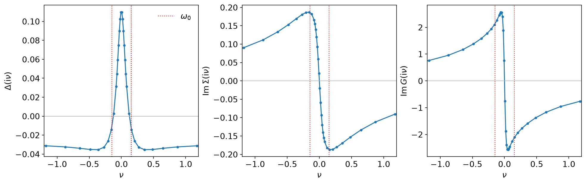
The gap is \(\Delta(\mathrm{i}\pi T) = 0.1098\), comfortably above \(\omega_0/2\), and it does not simply decay: it crosses zero just outside \(\pm\omega_0\) (the dotted lines) and reaches \(-0.0353\) before flattening out at \(-0.0292\). That negative tail is the Coulomb pseudopotential mechanism — the repulsion is pushed up to frequencies where the phonon no longer helps, and the low-frequency gap is left positive.
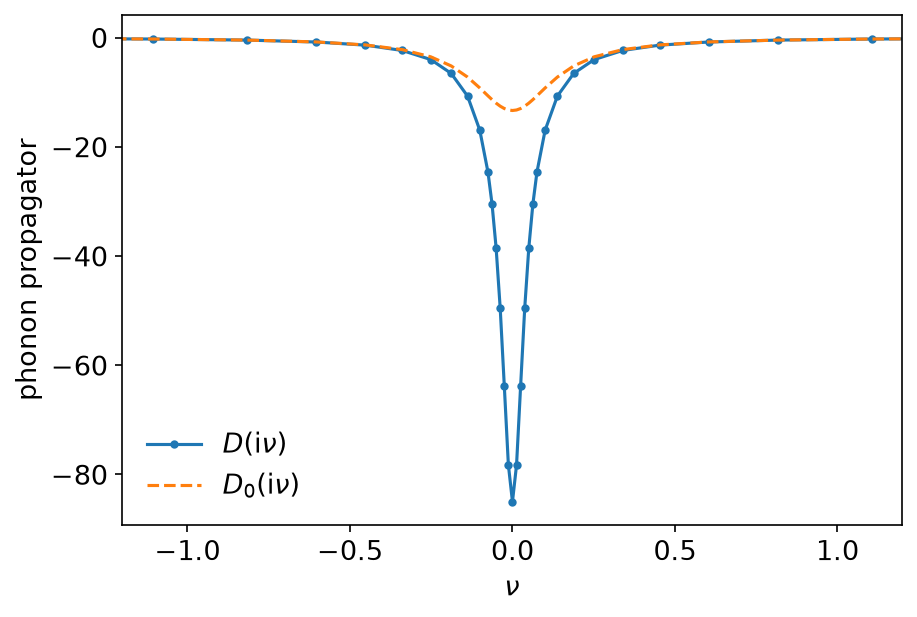
The phonon the electrons hand back is much softer than the one they were given: \(\mathcal{D}(0) = -85.0\) against a bare \(\mathcal{D}_0(0) = -2/\omega_0 = -13.3\), a factor of 6.4. For bosonic frequencies \(|\omega| \gtrsim 2\omega_0\) the two are indistinguishable.
Compactness, checked
The reason all of this fits in 45 numbers is the same reason it fits in the basis at all, and the anomalous Green’s function makes the point cleanly:
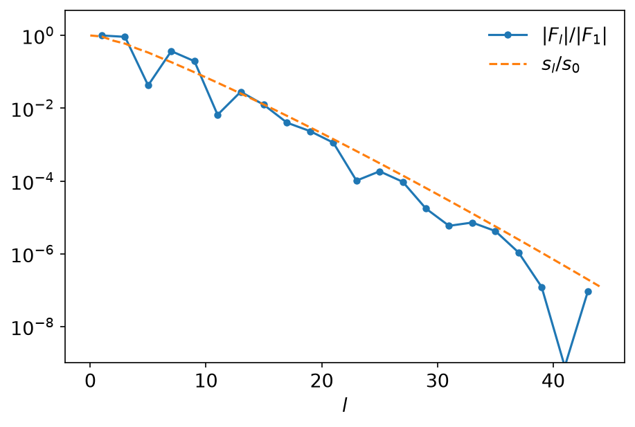
\(F\) is even in \(\nu\), so only odd \(l\) carry weight — the even coefficients sit at \(10^{-15}\), which is the round-off of the transform. What is left tracks \(s_l/s_0\) over about seven orders of magnitude (down to \(1.3\times10^{-7}\)) and stops where the expansion was truncated. A Matsubara sum reaching \(\nu = \pm 34.7\), which is where the sampling frequencies end, would have needed thousands of points to say the same thing.
The specific heat across the transition
The internal energy is a sum of three Matsubara sums, two fermionic and one
bosonic. In the basis each is a fit followed by one evaluation at
\(\tau = 0\), the same trick the TPSC sum rules use; the constant that the
basis cannot represent (\(\mathrm{i}\nu G \to 1\)) is subtracted before the
fit. Which side of \(\tau = 0\) is meant needs care. The textbook
convergence factor \(e^{\mathrm{i}\nu 0^+}\) selects \(\tau \to 0^-\), but
evaluate_tau(&[0.0]) reads \(+0.0\) as \(\tau = 0^+\), so the program
computes the \(0^+\) value. The two differ by the \(1/\mathrm{i}\nu\)
coefficient of the fitted function, and in this model that coefficient
vanishes (\(\mu = 0\), a symmetric \(\rho\), and \(\Sigma \to 0\) at large
\(\nu\)): evaluating at \(-0.0\), which the library reads as \(0^-\),
changes the two fermionic sums by about \(10^{-14}\). Away from half filling
the \(0^-\) side would have to be requested explicitly. The bosonic phonon
term is continuous at \(\tau = 0\); following the notebook, it is read at the
smallest positive sampling time \(\tau_0\).
The temperature derivative of the internal energy is the specific heat, so
eliashberg_holstein_scan solves the model twice at each of ten
temperatures — at \(T\) and at \(T + 10^{-5}\) — and takes the difference
quotient. At the stronger coupling \(\lambda_0 = 0.175\) the transition
falls inside \(T \in [0.009, 0.013]\).
The sweep holds \(\Lambda = \beta\omega_\mathrm{max} = 555.6\) fixed, so one expansion serves all twenty solves and the basis stays 36 functions throughout — which is what makes it safe to start each solve from the solution before it:
    let lambda_ir = WMAX / T_MIN;
    let (kernel, sve) = sve_for(1.0 / T_MIN, lambda_ir * T_MIN, EPS)?;
// ...
    for &temperature in &temperatures {
        let beta = 1.0 / temperature;
        let bases = Bases::from_sve(kernel, sve.clone(), beta, EPS)?;
        // ... start from the previous Σ and Δ ...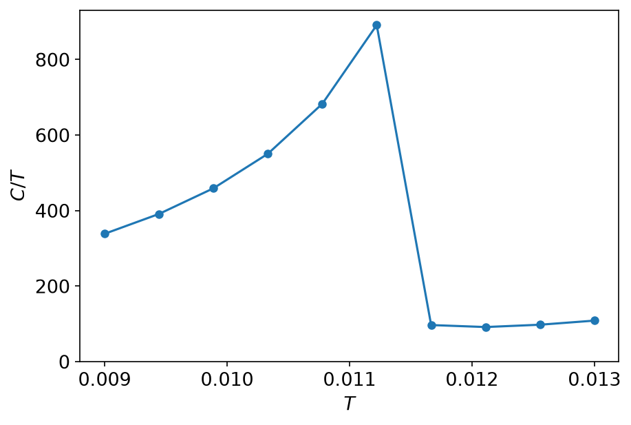
\(C/T\) climbs from 338 at \(T = 0.009\) to 891 at \(T = 0.011222\) and then falls off a cliff, to 96.7 one step later: the superconducting transition sits between those two temperatures. Above it \(C/T\) is flat and small, which is the normal state of a weakly coupled metal. The approach to the transition is also where the loop works hardest — 4476 iterations at the last superconducting point, against a dozen well above \(T_c\), the usual critical slowing down of a self-consistent solver.
Beyond the imaginary axis
The gap function here is known only at the sampling frequencies. The real-frequency gap \(\Delta(\omega)\) and the density of states of the superconductor need analytic continuation: see analytic continuation, sparse modeling and MiniPole. The DLR gives a pole representation of the same functions on the imaginary axis.
Running it
From docs/tutorial-code:
$ cargo run --profile ci --bin eliashberg_holstein
$ cargo run --profile ci --bin eliashberg_holstein_scan
$ uv run --project ../plotting python ../plotting/eliashberg_holstein_plot.py
eliashberg_holstein is one solve and takes well under a second;
eliashberg_holstein_scan is twenty solves, several of them slow, and takes a
couple of seconds. The starting self-energy is read from a committed noise
file rather than drawn at random, so that the Rust program and the Python
notebook start from the same numbers and the repository’s checks can compare
them.
Key API pieces
From sparse-ir:
| What you want | What to call |
|---|---|
| both statistics from one expansion | compute_sve, then FiniteTempBasis::from_sve_result for Fermionic and Bosonic |
| \(u^F_l(0^+)\) for a Matsubara sum | Basis::evaluate_tau(&[0.0]) (\(+0.0\) means \(0^+\), \(-0.0\) means \(0^-\)) |
| fits and evaluations at the sampling points | TauSampling, MatsubaraSampling (wrapped by IrMesh) |
From the tutorial crate (docs/tutorial-code/src):
| What you want | Tutorial helper |
|---|---|
| both bases and meshes from one expansion | Bases::new, or sve_for then Bases::from_sve |
| one pass of the loop | IrMesh::wn_to_tau, multiply, IrMesh::tau_to_wn |
| \(G(\beta - \tau) = -G(-\tau)\) on the sampling grid | IrMesh::reverse_tau |
| a Matsubara sum through the basis | IrMesh::wn_to_l, then evaluate_rows with \(u^F_l(0^+)\) |
| an integral over a density of states | gauss_legendre from tutorial::quad |
| the same basis at every temperature | fix \(\Lambda\) and vary \(\beta\) |