Discrete Lehmann Representation

Theory

We explain how to transform expansion coefficients in IR to the discrete Lehmann representation (DLR) [1]. In sparse-ir, we choose poles based on the exrema of \(V_l(\omega)\) [2] (In the original paper [1], a more systematic way is proposed). We model the spectral function as

\[ \rho(\omega) = \sum_{p=1}^L c_p \delta(\omega - \bar{\omega}_p), \]

where sampling frequencies \(\{\bar{\omega}_1, \cdots, \bar{\omega}_{L}\}\) are chosen to the extrema of \(V'_{L-1}(\omega)\). This choice is heuristic but allows us a numerically stable transform between \(\rho_l\) and \(c_p\) through the relation

\[ \rho_l = \sum_{p=1}^L \boldsymbol{V}_{lp} c_p, \]

where the matrix \(\boldsymbol{V}_{lp}~[\equiv V_l(\bar{\omega}_p)]\) is well-conditioned. As a result, in SPR, the Green’s function is represented as

\[ G(\mathrm{i}\omega_n) = \sum_{p=1}^L \frac{c_p}{\mathrm{i}\omega_n - \bar{\omega}_p}. \]

[1] J. Kaye, K. Chen, O. Parcollet, Phys. Rev. B 105, 235115 (2022).
[2] H. Shinaoka et al., arXiv:2106.12685v2.

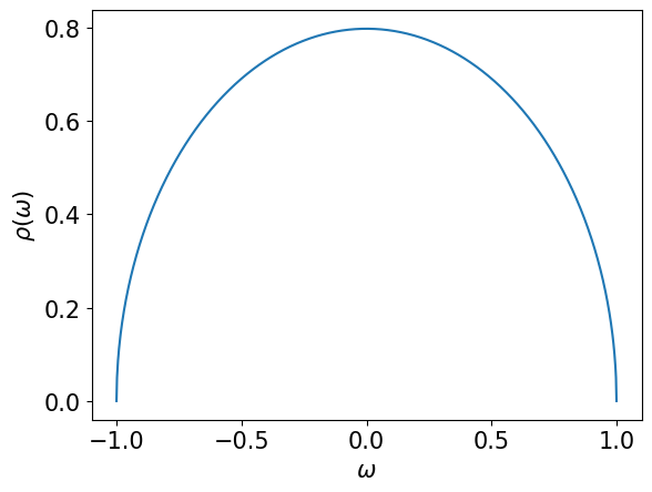
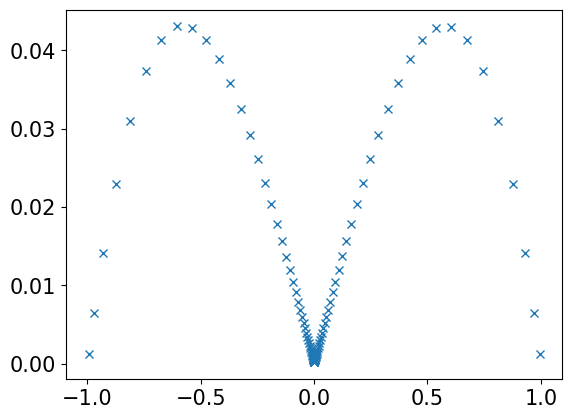
We consider the semi circular DOS

\[ \rho(\omega) = \sqrt{\frac{2}{\pi}} \sqrt{1-\omega^2}. \]

The corresponding Green’s function is given by

\[ G(\mathrm{i}\omega_n) = \int_{-1}^1 \mathrm{d}\omega \frac{\rho(\omega)}{\mathrm{i}\omega_n - \omega}. \]

The Green’s function is expanded in IR as

\[ G_l = - S_l \int_{-1}^1 \mathrm{d}\omega \rho(\omega) V_l(\omega). \]

Below, we demonstrate how to transform \(G_l\) to the DLR coefficients \(c_p\).

import numpy as np
from sparse_ir import FiniteTempBasis, MatsubaraSampling
from sparse_ir.dlr import DiscreteLehmannRepresentation

%matplotlib inline
from matplotlib import pyplot as plt
plt.rcParams['font.size'] = 15

Implementation

Create basis object

wmax = 1.0
lambda_ = 1e+4
beta = lambda_/wmax

basis = FiniteTempBasis("F", beta, wmax, eps=1e-15)
print(basis.size)

104

Setup model

rho = lambda omega: np.sqrt(1-omega**2)/np.sqrt(0.5*np.pi)

omega = np.linspace(-wmax, wmax, 1000)
plt.xlabel(r'$\omega$')
plt.ylabel(r'$\rho(\omega)$')
plt.plot(omega, rho(omega))
plt.show()

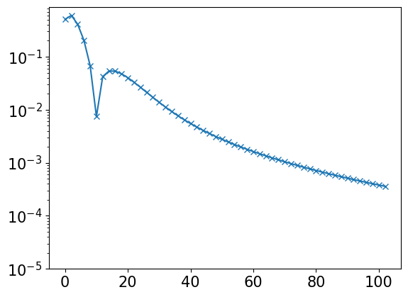
rhol = basis.v.overlap(rho)
ls = np.arange(basis.size)
plt.semilogy(ls[::2], np.abs(rhol)[::2], marker="x")
plt.ylim([1e-5, None])
plt.show()

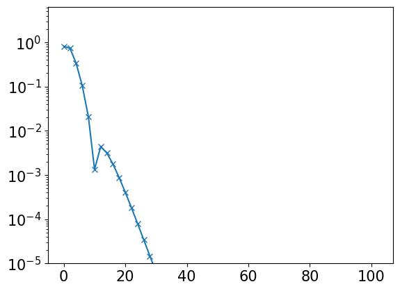
gl = - basis.s * rhol
plt.semilogy(ls[::2], np.abs(gl)[::2], marker="x")
plt.ylim([1e-5, None])
plt.show()

Create a DLR object and perform transformation

dlr = DiscreteLehmannRepresentation(basis)

# To DLR
g_dlr = dlr.from_IR(gl)

plt.plot(dlr.sampling_points, g_dlr, marker="x", ls="")
plt.show()

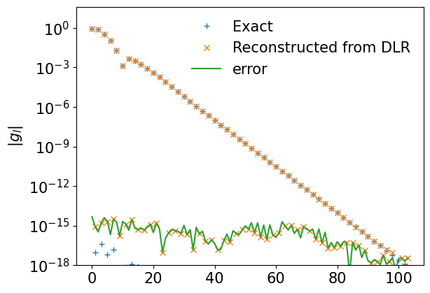
# Transform back to IR from SPR
gl_reconst = dlr.to_IR(g_dlr)

plt.semilogy(np.abs(gl), label="Exact", ls="", marker="+")
plt.semilogy(np.abs(gl_reconst), label="Reconstructed from DLR", ls="", marker="x")
plt.semilogy(np.abs(gl-gl_reconst), label="error")
plt.ylim([1e-18,None])
plt.ylabel("$|g_l|$")
plt.legend(loc="best", frameon=False)
plt.show()

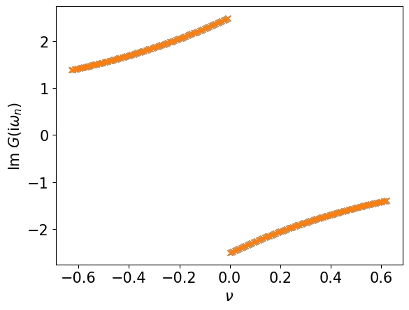
Evaluation on Matsubara frequencies

v = 2*np.arange(-1000, 1000, 10) + 1
iv = 1j * v * (np.pi/beta)

transmat = 1/(iv[:,None] - dlr.sampling_points[None,:])
giv = transmat @ g_dlr

giv_exact = MatsubaraSampling(basis, v).evaluate(gl)

plt.plot(iv.imag, giv_exact.imag, ls="", marker="x", label="Exact")
plt.plot(iv.imag, giv.imag, ls="", marker="x", label="Reconstructed from SPR")
plt.xlabel(r"$\nu$")
plt.ylabel(r"Im $G(\mathrm{i}\omega_n)$")

plt.show()