Sparse sampling

In this page, we describe how to infer IR expansion coefficients using the sparse-sampling techiniques.

import sparse_ir
import numpy as np
%matplotlib inline
import matplotlib.pyplot as plt
plt.rcParams['font.size'] = 15

Setup

We consider a semicircular spectral modeli (full bandwidth of 2):

\[ \rho(\omega) = \frac{2}{\pi}\sqrt{1-\omega^2}. \]

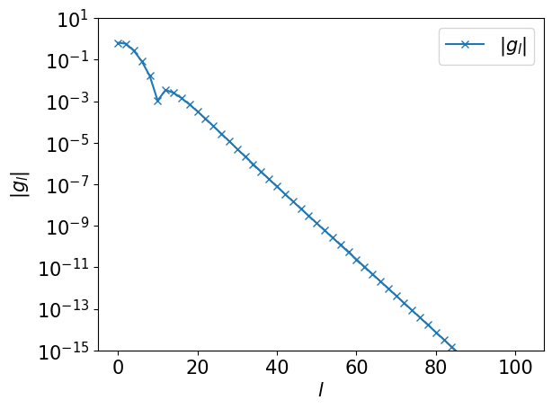
First, we compute the numerically exact expansion coefficients \(g_l\). Below, we plot the data for even \(l\).

def rho(omega):
    if np.abs(omega) < 1:
        return (2/np.pi) * np.sqrt(1-omega**2)
    else:
        return 0.0

beta = 10000
wmax = 1
basis = sparse_ir.FiniteTempBasis("F", beta, wmax, eps=1e-15)

rhol = basis.v.overlap(rho)
gl = - basis.s * rhol

ls = np.arange(basis.size)
plt.semilogy(ls[::2], np.abs(gl[::2]), marker="x", label=r"$|g_l|$")
plt.xlabel(r"$l$")
plt.ylabel(r"$|g_l|$")
plt.ylim([1e-15, 10])
plt.legend()
plt.show()

From sampling times

We first create a TauSampling object for the default sampling times.

smpl_tau = sparse_ir.TauSampling(basis)
print("sampling times: ", smpl_tau.sampling_points)
print("Condition number: ", smpl_tau.cond)

sampling times:  [6.47259411e-02 3.41743000e-01 8.43021447e-01 1.57374357e+00
 2.54146656e+00 3.75645685e+00 5.23203838e+00 6.98503912e+00
 9.03635582e+00 1.14116536e+01 1.41422159e+01 1.72659575e+01
 2.08286083e+01 2.48850703e+01 2.95009414e+01 3.47541980e+01
 4.07370279e+01 4.75578203e+01 5.53433349e+01 6.42411056e+01
 7.44221521e+01 8.60840959e+01 9.94547772e+01 1.14796470e+02
 1.32410787e+02 1.52644359e+02 1.75895379e+02 2.02621103e+02
 2.33346379e+02 2.68673315e+02 3.09292122e+02 3.55993176e+02
 4.09680252e+02 4.71384769e+02 5.42280708e+02 6.23699556e+02
 7.17144194e+02 8.24299996e+02 9.47040430e+02 1.08742317e+03
 1.24767097e+03 1.43012945e+03 1.63719162e+03 1.87117715e+03
 2.13415420e+03 2.42769528e+03 2.75256828e+03 3.10838360e+03
 3.49324565e+03 3.90348920e+03 4.33360019e+03 4.77640949e+03
 5.22359051e+03 5.66639981e+03 6.09651080e+03 6.50675435e+03
 6.89161640e+03 7.24743172e+03 7.57230472e+03 7.86584580e+03
 8.12882285e+03 8.36280838e+03 8.56987055e+03 8.75232903e+03
 8.91257683e+03 9.05295957e+03 9.17570000e+03 9.28285581e+03
 9.37630044e+03 9.45771929e+03 9.52861523e+03 9.59031975e+03
 9.64400682e+03 9.69070788e+03 9.73132669e+03 9.76665362e+03
 9.79737890e+03 9.82410462e+03 9.84735564e+03 9.86758921e+03
 9.88520353e+03 9.90054522e+03 9.91391590e+03 9.92557785e+03
 9.93575889e+03 9.94465667e+03 9.95244218e+03 9.95926297e+03
 9.96524580e+03 9.97049906e+03 9.97511493e+03 9.97917139e+03
 9.98273404e+03 9.98585778e+03 9.98858835e+03 9.99096364e+03
 9.99301496e+03 9.99476796e+03 9.99624354e+03 9.99745853e+03
 9.99842626e+03 9.99915698e+03 9.99965826e+03 9.99993527e+03]
Condition number:  51.830544391655934

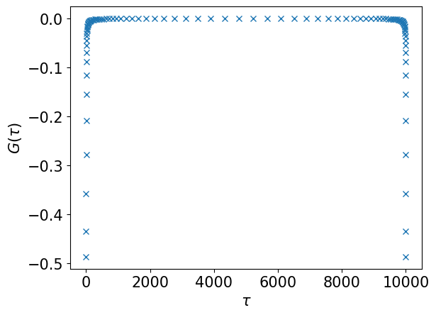
The condition number is around 50, indicating that 1–2 significant digits may be lost in a fit from the sampling times. Let us fit from the sampling times!

# Evaluate G(τ) on the sampling times
gtau_smpl = smpl_tau.evaluate(gl)
plt.plot(smpl_tau.sampling_points, gtau_smpl, marker="x", ls="")
plt.xlabel(r"$\tau$")
plt.ylabel(r"$G(\tau)$")
plt.show()

# Fit G(τ) on the sampling times
gl_reconst_from_tau = smpl_tau.fit(gtau_smpl)

From sampling frequencies

We create a MatsubaraSampling object for the default sampling frequencies.

smpl_matsu = sparse_ir.MatsubaraSampling(basis)
print("sampling frequencies: ", smpl_matsu.sampling_points)
print("Condition number: ", smpl_matsu.cond)

sampling frequencies:  [-44377 -14981  -8743  -6213  -4765  -3733  -3089  -2523  -2093  -1797
  -1513  -1315  -1117   -975   -859   -729   -623   -547   -469   -411
   -361   -309   -267   -233   -205   -177   -153   -133   -115   -101
    -87    -75    -65    -57    -49    -43    -37    -33    -29    -25
    -23    -21    -19    -17    -15    -13    -11     -9     -7     -5
     -3     -1      1      3      5      7      9     11     13     15
     17     19     21     23     25     29     33     37     43     49
     57     65     75     87    101    115    133    153    177    205
    233    267    309    361    411    469    547    623    729    859
    975   1117   1315   1513   1797   2093   2523   3089   3733   4765
   6213   8743  14981  44377]
Condition number:  210.8802635675076

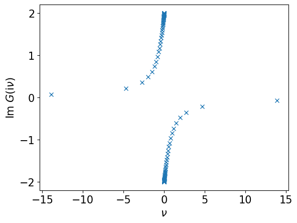
The condition number is slightly larger than that for the sampling times.

# Evaluate G(iv) on the sampling frequencies
giv_smpl = smpl_matsu.evaluate(gl)
plt.plot((np.pi/beta)*smpl_matsu.wn, giv_smpl.imag, marker="x", ls="")
plt.xlabel(r"$\nu$")
plt.ylabel(r"Im $G(\mathrm{i}\nu)$")
plt.show()

# Fit G(τ) on the sampling times
gl_reconst_from_matsu = smpl_matsu.fit(giv_smpl)

Comparison with exact results

We now compare the reconstructed expansion coefficients with the exact one. For clarity, we plot only the data for even \(l\).

plt.semilogy(ls[::2], np.abs(gl[::2]), marker="", ls="-", label="Exact")
plt.semilogy(ls[::2], np.abs(gl_reconst_from_tau[::2]), marker="x", label="from sampling times")
plt.semilogy(ls[::2], np.abs(gl_reconst_from_matsu[::2]), marker="+", label="from sampling frequencies")
plt.xlabel(r"$l$")
plt.ylabel(r"$|g_l|$")
plt.ylim([1e-17, 10])
plt.legend(frameon=False)
plt.show()

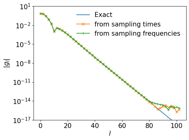
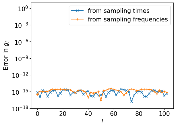
We saw a perfect match! Let us plot the differences from the exact one.

plt.semilogy(ls[::2], np.abs((gl_reconst_from_tau-gl)[::2]), marker="x", label="from sampling times")
plt.semilogy(ls[::2], np.abs((gl_reconst_from_matsu-gl)[::2]), marker="+", label="from sampling frequencies")
plt.xlabel(r"$l$")
plt.ylabel(r"Error in $g_l$")
plt.ylim([1e-18, 10])
plt.legend()
plt.show()