Two-particle self-consistency
Ported from the Python notebook
TPSC_py.ipynb
of the sparse-ir tutorials,
whose author is Niklas Witt. The programs that produced every number and
figure on this page are docs/tutorial-code/src/bin/tpsc.rs and
docs/tutorial-code/src/bin/tpsc_scan.rs; the solver is in
docs/tutorial-code/src/tpsc.rs, and the code below is included from there.
The previous page iterated a self-consistency loop thousands of times. This one does not iterate at all: the two-particle self-consistent approach fixes its vertices by solving two scalar equations, and the whole calculation is a single pass through the basis with a pair of root searches in the middle.
Vertices from sum rules
TPSC starts where RPA starts, with the irreducible susceptibility of the square lattice at half bandwidth \(4t\),
\[ \chi^0(\mathrm{i}\omega, q) ;=; -\frac{1}{N_k}\sum_{k} \int_0^\beta \mathrm{d}\tau; \mathrm{e}^{\mathrm{i}\omega\tau}, G(\tau, k), G(-\tau, k - q), \]
with \(\mathrm{i}\omega\) a bosonic Matsubara frequency (even reduced index) and \(\mathrm{i}\nu\) a fermionic one (odd), as in the conventions, and dresses it in the usual geometric way,
\[ \chi_\mathrm{sp} = \frac{\chi^0}{1 - U_\mathrm{sp}\chi^0}, \qquad \chi_\mathrm{ch} = \frac{\chi^0}{1 + U_\mathrm{ch}\chi^0}. \]
What is different is where \(U_\mathrm{sp}\) and \(U_\mathrm{ch}\) come from. RPA sets both to the bare \(U\) and is done. TPSC instead demands that the two susceptibilities satisfy the local sum rules exactly,
\[ \frac{2}{N_k\beta}\sum_{q,\omega} \chi_\mathrm{sp}(\mathrm{i}\omega, q) = n - 2\langle n_\uparrow n_\downarrow\rangle, \qquad \frac{2}{N_k\beta}\sum_{q,\omega} \chi_\mathrm{ch}(\mathrm{i}\omega, q) = n + 2\langle n_\uparrow n_\downarrow\rangle - n^2, \]
where \(n\) on the right is the filling, and closes the first of them with the Kanamori–Brueckner ansatz \(\langle n_\uparrow n_\downarrow\rangle = \tfrac14 (U_\mathrm{sp}/U),n^2\). That makes the spin rule an equation in \(U_\mathrm{sp}\) alone; the double occupancy that comes out of it then makes the charge rule an equation in \(U_\mathrm{ch}\) alone. Two one-dimensional root searches, no loop.
The sums on the left are the reason this page belongs in a basis tutorial. A sum over every bosonic Matsubara frequency is, in the basis, the value of the zone-averaged susceptibility at \(\tau = 0\): fit once, evaluate once.
    let chi = rpa(chi_0, vertex);
    let averaged: Vec<Complex64> = (0..lattice.mesh_b().n_wn())
        .map(|i| chi[i * nk..(i + 1) * nk].iter().sum::<Complex64>() / nk as f64)
        .collect();
    let coefficients = lattice.mesh_b().wn_to_l(&averaged, 1)?;
    Ok(evaluate_rows(lattice.ub_at_zero(), &coefficients, 1)[0].re)
Each evaluation of the sum rule costs one fit of 31 sampling points onto 30 basis functions and one evaluation of \(u^B_l(0)\), so putting it inside a root search (Brent’s method) is affordable. With a truncated Matsubara sum it would not be: the tail of \(\chi\) decays as \(1/\omega^2\) and the sum rule is precisely the quantity that tail controls.
\(\chi^0\) itself is the same convolution as on the GW page, built as a product in \((\tau, r)\):
    let grt = {
        let gkt = lattice.mesh_f().wn_to_tau(gkio, nk)?;
        lattice.grid().k_to_r(&gkt)
    };
    let reversed = lattice.mesh_f().reverse_tau(&grt, nk);
    let product: Vec<Complex64> = grt.iter().zip(&reversed).map(|(a, b)| a * b).collect();
    let in_momentum = lattice.grid().r_to_k(&product);
    lattice.mesh_b().tau_to_wn(&in_momentum, nk)
The one subtlety is reverse_tau. It returns \(G(\beta - \tau)\): the
sampling points read backwards together with the fermionic sign,
\(G(\beta - \tau) = -G(-\tau)\). The product is therefore
\(-G(\tau)G(-\tau)\), which is where the minus sign in \(\chi^0\) comes
from. Reading the points backwards works because the sampling times lie on
\([-\beta/2, \beta/2]\) and are (nearly) symmetric about \(0\) — a
point at \(\beta/2\) is matched with its image one period away;
tau_reversal panics if some \(-\tau\) is missing. And the fermionic and
bosonic \(\tau\) grids coincide, because the logistic kernel gives both
statistics the same \(u_l(\tau)\); Bases::from_sve asserts that the two
grids are equal. That is what lets the product, sampled on fermionic times,
be fitted with the bosonic sampling object.
With the two vertices fixed, the self-energy is one more product in \((\tau, r)\),
\[ \Sigma(\tau, r) = V(\tau, r), G(\tau, r), \qquad V = \frac{U}{4}\left(3U_\mathrm{sp}\chi_\mathrm{sp} + U_\mathrm{ch}\chi_\mathrm{ch}\right), \]
built from the non-interacting \(G\), after which \(\mu\) is refixed for the interacting \(G\). As on the FLEX page, the instantaneous Hartree shift is left out of \(V\) and absorbed into \(\mu\).
One solve at U = 4
tpsc takes a \(24 \times 24\) lattice at \(\beta = 10\), filling
\(n = 0.85\), \(U = 4\) and \(\varepsilon = 10^{-10}\). The basis has 30
functions for each statistics, giving 30 \(\tau\) points, 30 fermionic and
31 bosonic frequencies — the entire frequency content of a lattice problem at
\(\beta\omega_\mathrm{max} = 100\).
The vertices come out as
\[ U_\mathrm{sp} = 2.1011 ;<; U = 4 ;<; U_\mathrm{ch} = 7.6738, \]
which is the qualitative statement TPSC exists to make: spin fluctuations screen the interaction in the spin channel and anti-screen it in the charge channel, and RPA’s \(U_\mathrm{sp} = U\) overshoots badly. The double occupancy is \(0.0949\), well below the uncorrelated \((n/2)^2 = 0.1806\).
Note also \(U_\mathrm{crit} = 1/\max\chi^0 = 2.3821\). The spin sum rule has
no solution above it — the RPA denominator would change sign — so
\(U_\mathrm{sp}\) is bounded by \(U_\mathrm{crit}\) no matter how large
\(U\) grows. That bound is what enforces the Mermin–Wagner theorem here, and
a request that would violate it is reported as TpscError::Ordered rather
than producing a number.
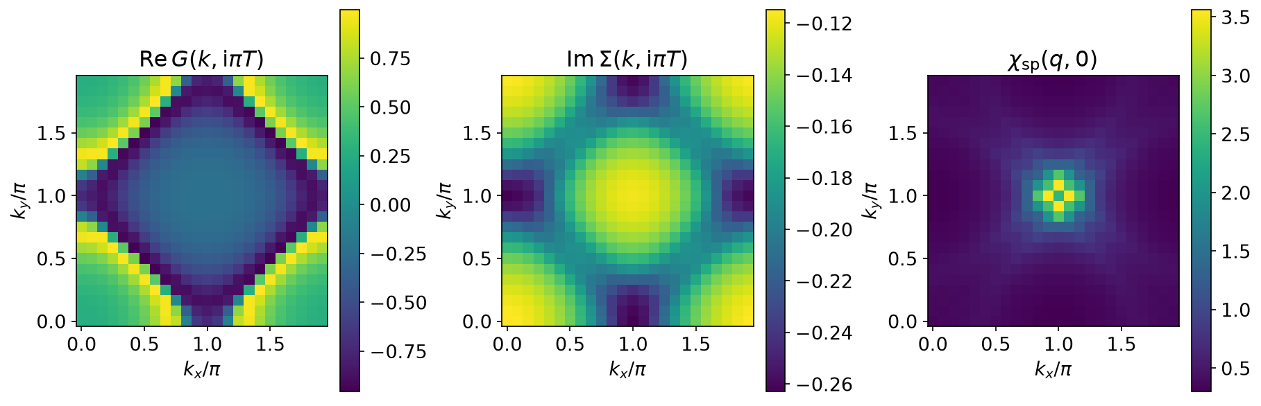
The zeroth Matsubara slice shows a Fermi surface in \(\mathrm{Re},G\), \(|\mathrm{Im},\Sigma|\) largest near the antinodes \((\pi, 0)\) — the beginning of the pseudogap — and \(\chi_\mathrm{sp}\) piled up around \(M = (\pi,\pi)\).
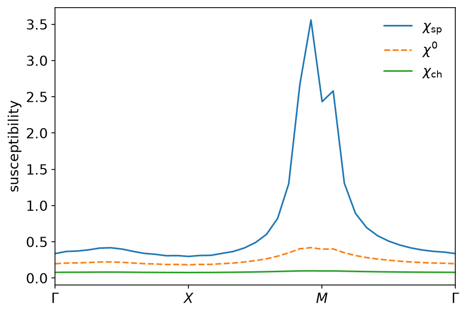
Along the high-symmetry path the ordering \(\chi_\mathrm{sp} > \chi^0 > \chi_\mathrm{ch}\) holds everywhere, and the enhancement is strongly momentum-selective: a factor of about 8.5 at the peak against 1.7 at \(\Gamma\). The peak is not at \(M\). At \(n = 0.85\) the system is doped, nesting is incommensurate, and the maximum sits one grid step away at \((\pi, 11\pi/12)\) with the value \(3.559\) against \(2.434\) at \(M\) itself.
Scanning U
tpsc_scan repeats the solve at half filling and \(T = 0.4\) for 51 values
of \(U\) from \(0.01\) to \(5\), which is the sweep behind Fig. 2 of
Y. M. Vilk and A.-M. S. Tremblay, J. Phys. I France 7, 1309 (1997).
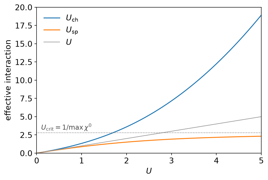
\(U_\mathrm{crit} = 2.7789\) is a property of \(\chi^0\), which does not depend on \(U\), and so is the same at every point of the scan. \(U_\mathrm{sp}\) rises from \(0.00999\) and flattens against that ceiling, reaching \(2.318\), i.e. \(83%\) of \(U_\mathrm{crit}\), at \(U = 5\). \(U_\mathrm{ch}\) has no such bound and runs away to \(18.9\). Between them the double occupancy falls from \(0.2497\) — the uncorrelated \(1/4\) — to \(0.1159\).
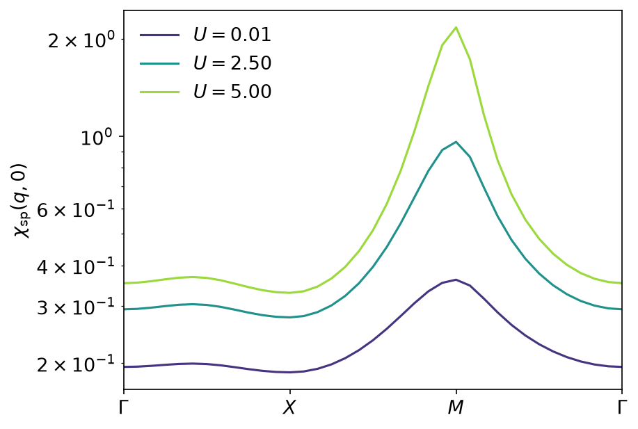
The susceptibility at half filling does peak at \(M\), and it grows by a factor of six there between \(U = 0.01\) and \(U = 5\) while barely doubling at \(\Gamma\). The saturating \(U_\mathrm{sp}\) is what keeps that growth finite: in RPA the same sweep would have diverged long before \(U = 5\).
Beyond the imaginary axis
The output here is \(G\), \(\Sigma\) and \(\chi\) on the sampling frequencies. For real-frequency spectra — the pseudogap in \(A(k,\omega)\), say — see analytic continuation, sparse modeling and MiniPole; for a compact pole representation of the same data, see the DLR.
Running it
From docs/tutorial-code:
$ cargo run --profile ci --bin tpsc
$ cargo run --profile ci --bin tpsc_scan
$ uv run --project ../plotting python ../plotting/tpsc_plot.py
Both programs are fast. tpsc is a single solve of a \(24\times24\)
lattice; tpsc_scan is 51 of them at a smaller basis and finishes in a
fraction of a second. The repository’s checks compare the outputs with the
Python notebook; they also assert that the \(n = 0.85\) peak lies on
\(k_x = \pi\) within one grid step of \(M\) (not at \(M\)) and that
\(U_\mathrm{crit}\) is constant along the scan.
Key API pieces
From sparse-ir:
| What you want | What to call |
|---|---|
| one SVE for both statistics | compute_sve, then FiniteTempBasis::from_sve_result twice |
| \(u_l(0)\), the row that turns a Matsubara sum into an evaluation | Basis::evaluate_tau(&[0.0]) |
| fits and evaluations at the sampling points | TauSampling, MatsubaraSampling (wrapped by IrMesh) |
From the tutorial crate (docs/tutorial-code/src):
| What you want | Tutorial helper |
|---|---|
| a Matsubara sum over all frequencies | IrMesh::wn_to_l, then evaluate_rows with \(u^B_l(0)\) |
| \(G(\beta - \tau) = -G(-\tau)\) on the sampling grid | IrMesh::reverse_tau |
| a fermionic product fitted as bosonic | IrMesh::wn_to_tau on one mesh, IrMesh::tau_to_wn on the other |
| both bases and meshes from one SVE | sve_for, Bases::from_sve (inside Lattice::new) |
| \(\chi^0\) as a real-space product | MomentumGrid::k_to_r, MomentumGrid::r_to_k |
| solving a sum rule for a vertex | brent from tutorial::roots |