DMFT with an IPT solver
Ported from the Python notebook
DMFT_IPT_py.ipynb
of the sparse-ir tutorials,
whose author is Niklas Witt. The programs that produced every number and
figure on this page are docs/tutorial-code/src/bin/dmft_ipt.rs and
docs/tutorial-code/src/bin/dmft_ipt_scan.rs; the loop itself is in
docs/tutorial-code/src/dmft.rs, and the code below is included from there.
Every applied page so far computed something once. This one iterates: a self-consistency loop that goes through the basis twice per step, several thousand times over. That makes it the page where the basis has to be cheap, and the page where a symmetry the exact solution has, but the arithmetic only nearly has, decides what the loop converges to.
The model and the loop
Dynamical mean-field theory replaces a lattice problem by a single impurity in a bath that is fixed by demanding that the impurity’s Green’s function is the lattice’s local one. On the Bethe lattice, with the semicircular density of states
\[ \rho(\omega) = \frac{2}{\pi D^2}\sqrt{D^2 - \omega^2}, \qquad D = 2t_\star = 2, \]
the self-consistency condition collapses to one line,
\[ \mathcal{G}^{-1}(\mathrm{i}\nu) = \mathrm{i}\nu - t_\star^2 G_\mathrm{loc}(\mathrm{i}\nu), \]
and iterated perturbation theory approximates the impurity self-energy by the second-order diagram, which at half filling is just a cube in imaginary time:
\[ \Sigma(\tau) = U^2 \mathcal{G}(\tau)^3, \qquad G_\mathrm{loc}^{-1}(\mathrm{i}\nu) = \mathcal{G}^{-1}(\mathrm{i}\nu) - \Sigma(\mathrm{i}\nu). \]
\(\Sigma\) is local in \(\tau\) and the Dyson equation is local in \(\mathrm{i}\nu\), so each iteration is a round trip between the two representations — exactly what the basis is for:
            // Σ(τ) = U² 𝒢(τ)³, which is the whole impurity solver.
            let g_tau = self.mesh.wn_to_tau(&g_weiss, 1)?;
            let sigma_tau: Vec<Complex64> = g_tau.iter().map(|g| u * u * g * g * g).collect();
            let mut fresh = self.mesh.tau_to_wn(&sigma_tau, 1)?;
At \(\beta = 20\), \(\omega_\mathrm{max} = 2D = 4\) and \(\varepsilon = 10^{-15}\) the basis has 37 functions, with 37 sampling times and 38 sampling frequencies. That is the entire state of the calculation: 37 coefficients carry a function whose Matsubara tail reaches out to \(\nu \sim 10^2\), and the round trip is two small dense solves. Nothing in the loop grows with \(\beta\) except logarithmically, which is what makes a 5000-iteration run a matter of seconds.
The non-interacting starting point comes from the same basis. The spectral representation \(G^0(\mathrm{i}\nu) = \int\mathrm{d}\omega, \rho(\omega)/(\mathrm{i}\nu - \omega)\) becomes, in IR coefficients, \(g_l = -s_l \rho_l\) with \(\rho_l = \int\mathrm{d}\omega, v_l(\omega)\rho(\omega)\). The overlap \(\rho_l\) is computed by Gauss–Legendre quadrature after the substitution \(\omega = D\sin\theta\), which removes the square-root singularity at the band edges, so the result is exact to machine precision:
        let rho_l = shifted_semicircle_overlaps(&self.basis, 0.0, self.d, 1.0);
        let g_l: Vec<Complex64> = self
            .basis
            .s()
            .iter()
            .zip(&rho_l)
            .map(|(s, rho)| Complex64::new(-s * rho, 0.0))
            .collect();
        self.mesh.l_to_wn(&g_l, 1)
The mixing is the notebook’s: \(\Sigma \leftarrow 0.25,\Sigma_\mathrm{new}
- 0.75,\Sigma_\mathrm{old}\).
One step is not in the notebook. At half filling with a symmetric density of states the exact self-energy is particle-hole symmetric: \(\Sigma(\mathrm{i}\nu)\) is purely imaginary and odd in \(\nu\). The round trip through the basis preserves that only to rounding, so the loop projects each new self-energy back onto its symmetric part, \(\Sigma(\mathrm{i}\nu) \to \mathrm{i},\tfrac12[\mathrm{Im},\Sigma(\mathrm{i}\nu) - \mathrm{Im},\Sigma(-\mathrm{i}\nu)]\). The next section shows why that is not optional.
            if symmetry == Symmetry::ParticleHole {
                fresh = self.particle_hole_symmetric(&fresh);
            }
One solve at \(U = 5\)
Run the loop at \(U = 5\) with the notebook’s stopping rule — stop when the relative change of \(\Sigma\) falls below \(10^{-5}\) — and it stops at iteration 65, reporting
\[ Z = \left(1 - \frac{\partial,\mathrm{Im},\Sigma}{\partial \nu}\right)^{-1} \approx 0.263, \]
a quasiparticle weight of a quarter: a correlated metal. The derivative is a finite difference over the two lowest positive frequencies, \(\partial,\mathrm{Im},\Sigma/\partial\nu \approx [\mathrm{Im},\Sigma(\mathrm{i}\nu_3) - \mathrm{Im},\Sigma(\mathrm{i}\nu_1)] /(2\pi/\beta)\) (reduced indices \(n = 1, 3\)), and a negative \(Z\) is reported as zero. Here is that solution:
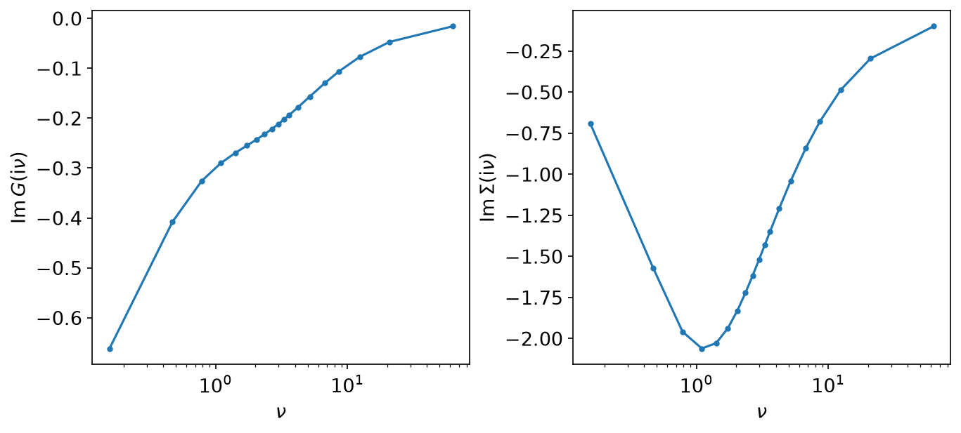
Left to run for 5000 iterations, the same loop settles on the same metal: the residual reaches \(10^{-16}\) by iteration 270 and stays there, and \(Z = 0.26307\) differs from the stopped run’s \(0.26310\) in the fifth digit, about what a threshold of \(10^{-5}\) on the change promises.
Now switch the projection off. Nothing else changes — same start, same mixing — and the run follows the symmetric one for 60 iterations, then leaves it:
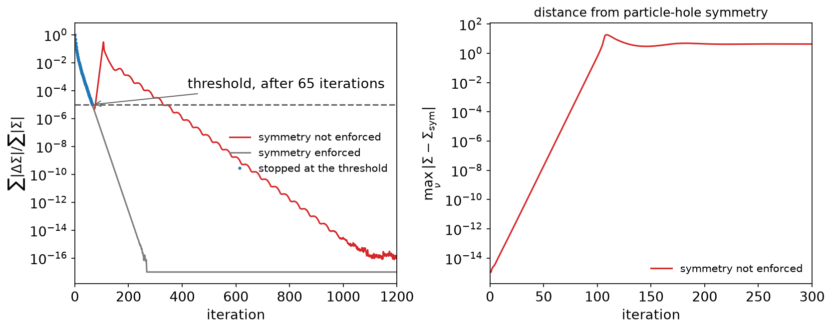
The right panel is the reason. The distance of \(\Sigma\) from its symmetric part starts at the \(10^{-15}\) of rounding and grows by about 40% per iteration, a straight line on the log scale, until it is of order one after 100 iterations. The symmetric metal is a fixed point of the loop, but an unstable one with respect to perturbations that break the symmetry, and rounding supplies such a perturbation at every step. The unprojected run then converges again (left panel, red) — to a state whose self-energy is far from particle-hole symmetric, which the exact solution of this half-filled model cannot be. Which broken state it reaches, and when it leaves, depends on the last bits of the arithmetic: two implementations, or two BLAS backends, generally land on different ones.
The moral is not specific to IR. A self-consistency loop converges to the fixed points that are stable under its own iteration, which need not be the physical ones; if the physical solution has a symmetry, impose it.
Scanning \(U\): the Mott transition and its hysteresis
dmft_ipt_scan sweeps \(U\) from 0 to 6.5 in 66 steps, three times:
- starting each \(U\) from the non-interacting \(G^0\);
- sweeping upwards, starting each \(U\) from the previous solution (the metal branch);
- sweeping downwards from \(U = 6.5\) (the insulator branch).
Every solve runs a fixed 5000 iterations with no stopping rule, so every point is a fixed point to machine precision rather than a snapshot on the way to one; the slowest, next to the edges of the coexistence window, are converged long before that.
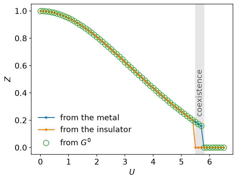
\(Z\) falls smoothly from 1 and then drops to zero, but not at the same \(U\) going up as coming down. The metal exists up to \(U = 5.7\) and is gone at 5.8, so \(U_{c2}\) lies between the two. Walking down, the insulator survives to \(U = 5.5\). In between both solutions are stable and which one you get depends on where you started: that shaded window is the first-order Mott transition. Its lower edge depends on how it is approached — started directly from the \(U = 6.5\) insulator instead of from its neighbour, the loop still finds an insulator at \(U = 5.3\) — which is the usual caveat about mapping a coexistence region with a simple iteration.
Starting from \(G^0\) lands on the metal branch wherever the metal exists —
the from_g0 and metal columns agree to \(10^{-15}\) across the whole
grid — which is why a naive scan sees only \(U_{c2}\) and misses the
hysteresis entirely.
The self-energies on either side make the distinction concrete:
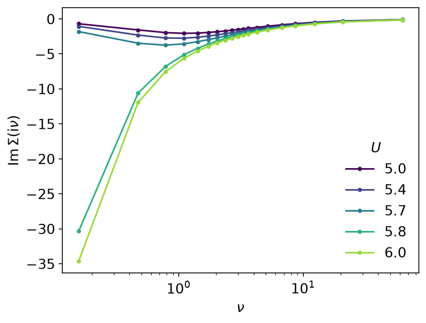
These are the solves started from \(G^0\), so they are on the metal branch wherever it exists. At \(U = 5.0, 5.4, 5.7\) \(\mathrm{Im},\Sigma\) turns back towards zero at the lowest frequencies, a Fermi liquid with a strongly reduced \(Z\). At \(U = 5.8\) and \(U = 6.0\) it diverges as \(\nu \to 0\), which is the pole at the Fermi level that opens the Mott gap.
Without the projection, this scan finds a “transition” between \(U = 3.4\) and \(3.5\) instead: there the symmetry-breaking instability of the previous section sets in within 5000 iterations, and the loop leaves the metal for a broken-symmetry state long before the metal ceases to exist.
Beyond the imaginary axis
Everything above lives on the imaginary axis. The contrast between the metal and the Mott insulator is most visible in the spectral function \(A(\omega)\) — a quasiparticle peak at \(\omega = 0\) against a gap between two Hubbard bands — and getting there from \(G(\mathrm{i}\nu)\) is analytic continuation. The IR coefficients \(g_l\) computed here are the natural input: see analytic continuation for regularised inversion of \(g_l = -s_l\rho_l\), sparse modeling for the \(\ell_1\)-regularised version, and MiniPole for a pole representation of \(G(\mathrm{i}\nu)\) from which \(A(\omega)\) can be read off.
Running it
From docs/tutorial-code:
$ cargo run --profile ci --bin dmft_ipt
$ cargo run --profile ci --bin dmft_ipt_scan
$ uv run --project ../plotting python ../plotting/dmft_ipt_plot.py
dmft_ipt takes about a second. dmft_ipt_scan is 198 self-consistent
solves of 5000 iterations each, which is closer to half a minute. The
binaries write CSV tables under docs/tutorial-code/data/; the plotting
script only reads them.
The repository checks these numbers against a Python version of the notebook’s loop with the same symmetry projection. The run without the projection is compared only by its shape, since where it ends up is decided by rounding.
Key API pieces
From sparse-ir:
| What you want | What to call |
|---|---|
| the fermionic IR basis at \(\beta\), \(\omega_\mathrm{max}\), \(\varepsilon\) | LogisticKernel::new, FiniteTempBasis::<_, Fermionic>::new |
| sampling in \(\tau\) and \(\mathrm{i}\nu\) | TauSampling::new, MatsubaraSampling::new (wrapped by IrMesh) |
| \(s_l\) and \(v_l(\omega)\) for \(g_l = -s_l\rho_l\) | basis.s(), basis.v() (get_knots, get_polyorder) |
| the reduced index of a sampling frequency | MatsubaraFreq::n |
From the tutorial crate (docs/tutorial-code/src):
| What you want | Tutorial helper |
|---|---|
| \(\tau \to \mathrm{i}\nu\) and back, once per iteration | IrMesh::tau_to_wn, IrMesh::wn_to_tau |
| \(\rho_l\) of a semicircle, by quadrature | shifted_semicircle_overlaps, then IrMesh::l_to_wn |
| \(\Sigma(\tau)\) for plotting | IrMesh::wn_to_l, then IrMesh::l_to_tau |
| the lowest Matsubara frequency | the position of \(n = 1\) in IrMesh::wn |