Orbital magnetic susceptibility
Ported from the Python notebook
orbital_magnetic_susceptibility_py.ipynb
of sparse-ir-tutorial,
whose authors are Soshun Ozaki and Takashi Koretsune. The program that
produced every number and figure on this page is
docs/tutorial-code/src/bin/orbital_magnetic_susceptibility.rs; the code below
is included from it.
The previous page used the basis to turn a Matsubara sum into one evaluation. This one does the same thing for a harder summand, and adds the other piece every multi-orbital calculation needs: a Hamiltonian that is a matrix at each momentum.
Theory
Orbital magnetism is what a vector potential coupled to the electron momentum induces. For a tight-binding model the susceptibility has a closed form in terms of the Green’s function and the derivatives of the Hamiltonian,
\[ \chi = T \sum_\nu \chi(\mathrm{i}\nu), \qquad \chi(\mathrm{i}\nu) = \frac{1}{N_k}\sum_{\boldsymbol{k}} \mathrm{Tr}\left[ \gamma_x G \gamma_y G \gamma_x G \gamma_y G
- \tfrac{1}{2}(\gamma_x G \gamma_y G + \gamma_y G \gamma_x G)\gamma_{xy} G \right], \]
with \(G = G(\mathrm{i}\nu, \boldsymbol{k})\), \(\gamma_i = \partial H_{\boldsymbol{k}} / \partial k_i\), \(\gamma_{xy} = \partial^2 H_{\boldsymbol{k}} / \partial k_x \partial k_y\), and \(\nu = \nu_n = n\pi/\beta\) running over the fermionic frequencies (\(n\) odd). The momentum sum is an average over the \(N_k\) points of the zone, so \(\chi\) is per unit cell. Units are \(e = \hbar = k_B = 1\) with \(t = a = 1\): the prefactor \(e^2/\hbar^2\) of the notebook’s formula is dropped. No spin factor is included, so \(\chi\) is for one spin species; multiply by 2 for spin-degenerate electrons. The formula is due to Gómez-Santos and Stauber, and to Raoux, Piéchon, Fuchs and Montambaux; its relation to Fukuyama’s continuum formula was settled by Ogata and Fukuyama and by Matsuura and Ogata.
The example computes it at \(T = 0.1\) (\(\beta = 10\)) on a \(200 \times 200\) momentum grid, for 91 chemical potentials from \(\mu = -4.5\) to \(4.5\). The basis uses \(\omega_\mathrm{max} = 10\) (\(\Lambda = 100\)) and \(\varepsilon = 10^{-10}\), which gives 30 functions:
const T_HOPPING: f64 = 1.0;
const LATTICE: f64 = 1.0;
const TEMPERATURE: f64 = 0.1;
const BETA: f64 = 1.0 / TEMPERATURE;
const WMAX: f64 = 10.0;
const EPS: f64 = 1e-10;
const NK_LIN: usize = 200;
/// The chemical potentials `χ` is scanned over, from −4.5 to 4.5.
const N_MU: usize = 91;
const MU_MIN: f64 = -4.5;
const MU_MAX: f64 = 4.5;
/// The chemical potential the sampled `χ(iν)` is written out at. Not μ = 0:
/// both lattices are particle-hole symmetric there and `χ(iν)` comes out
/// real, which would hide a mistake in its imaginary part.
const PROBE_MU: f64 = -1.0;
It is written entirely in Matsubara sums of products of Green’s functions, which is what makes it a good example. Here the summand is a product of three or four of them, not two:
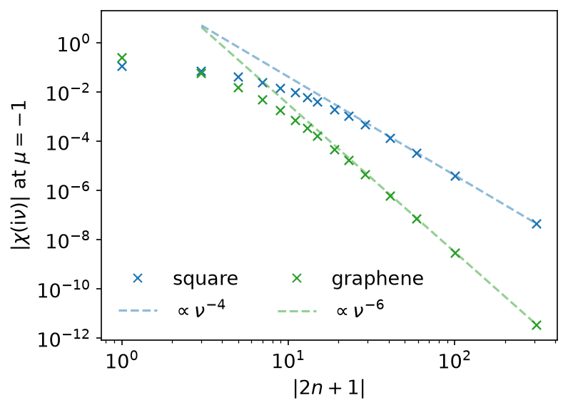
The square lattice falls off as \(\nu^{-4}\) — a dispersion that separates has no \(\gamma_{xy}\), so the three-Green’s-function term is absent entirely — and graphene, whose velocity matrices are purely off-diagonal in the site basis, as \(\nu^{-6}\). Thirty sampling frequencies hold all of it, and the sum is again
    // `T Σ_ν F(iν) = F(τ = 0)`: the Matsubara sum is the basis expansion read
    // at one point. This is the row of basis functions that reads it.
    let u_at_zero = basis.evaluate_tau(&[0.0])?;
        let coefficients = mesh.wn_to_l(&chi_iw, N_MU)?;
        let chi: Vec<f64> = evaluate_rows(&u_at_zero, &coefficients, N_MU)
            .iter()
            .map(|z| z.re)
            .collect();
with one column per chemical potential; there are 91 of them, fitted in one call.
Square lattice
One band makes every matrix in the formula a number and the trace a product, so the whole summand is two terms:
        for (i, &nu) in nu.iter().enumerate() {
            for (m, &mu) in mu.iter().enumerate() {
                let g = Complex64::new(-(ek - mu), nu).inv();
                let g2 = g * g;
                chi[i * n_mu + m] += gx * gx * gy * gy * g2 * g2 + gx * gy * gxy * g2 * g;
            }
        }
After the loop over momenta, the sum is divided by \(N_k\):
    // The k sum is an average over the zone: χ per unit cell.
    let nk = grid.len() as f64;
    chi.iter().map(|z| z / nk).collect()
\(\gamma_{xy}\) is identically zero here, and the second term with it; the example keeps it so that the code is the formula rather than a special case of it.
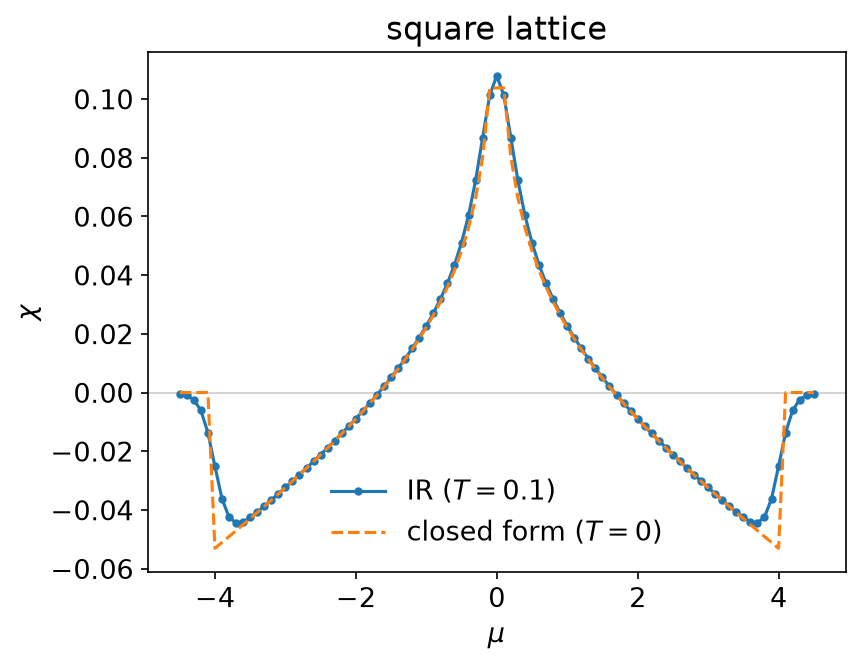
At \(T = 0\) the same quantity is known in closed form,
\[ \chi = -\frac{2}{3\pi^2}\left[E(m) - \frac{K(m)}{2}\right], \qquad m = 1 - \frac{\mu^2}{16}, \]
zero outside the band. sparse_ir_tutorial::elliptic computes \(K\) and
\(E\) from the arithmetic-geometric mean, which is a dozen lines and needs
no dependency. The two curves lie on top of each other to better than
\(10^{-3}\) for \(1 \le |\mu| \le 3\), and part company only where they
must: at the van Hove filling \(\mu = 0\), where the closed form diverges and
\(T = 0.1\) does not, and at the band edge, where the Fermi function rounds
the step off. Because of the divergence, the program leaves \(\mu = 0\) out of
the closed-form table.
Graphene
Two sites per cell make \(H_{\boldsymbol{k}}\) a 2×2 matrix, which has to be diagonalised before the Green’s function can be written down. In the eigenbasis \(G\) is diagonal, so the trace of four matrices becomes a product of 2×2 matrices whose columns are scaled by \(G\):
        let eigen = hamiltonian.eigen();
        // In the eigenbasis `G` is diagonal, so the traces below are products
        // of 2×2 matrices and two numbers rather than of four matrices.
        let [gx, gy, gxy] = velocities.map(|m| Hermitian2::rotate(&eigen, &m));
        for (i, &nu) in nu.iter().enumerate() {
            for (m, &mu) in mu.iter().enumerate() {
                let g = [
                    Complex64::new(-(eigen.values[0] - mu), nu).inv(),
                    Complex64::new(-(eigen.values[1] - mu), nu).inv(),
                ];
                let (xg, yg, xyg) = (
                    times_green(&gx, &g),
                    times_green(&gy, &g),
                    times_green(&gxy, &g),
                );
                let xy = product(&xg, &yg);
                let yx = product(&yg, &xg);
                chi[i * n_mu + m] += trace(&xy, &xy) + 0.5 * (trace(&xy, &xyg) + trace(&yx, &xyg));
            }
        }
Hermitian2 in sparse_ir_tutorial::linalg solves the 2×2 eigenproblem in
closed form rather than calling a general routine, because a general routine
is free to return the eigenvectors with any phase and the tutorial’s numbers
have to be reproducible. The susceptibility does not care about the phase:
it is a trace of rotated matrices.
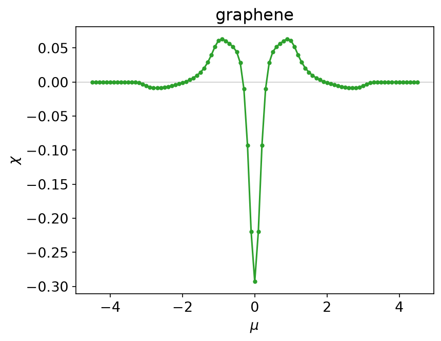
The result is the opposite of the square lattice: a sharp diamagnetic peak at the Dirac point, the delta function of the massless spectrum rounded by temperature, paramagnetic shoulders on either side, and nothing at all outside the band, which spans \(|\epsilon| \le 3t\).
Going further
This page uses only the IR basis and stays on the imaginary axis. For real-frequency output, see MiniPole, which fits a few poles to Matsubara data by ESPRIT, and Analytic continuation for why that step is ill posed. The DLR page shows the pole-based representation of imaginary-axis data.
Running it
From docs/tutorial-code:
$ cargo run --release --bin orbital_magnetic_susceptibility
The program writes CSV tables to
docs/tutorial-code/data/orbital_magnetic_susceptibility/. The figures are
drawn from those tables; from the repository root, run
uv run --project docs/plotting python docs/plotting/orbital_magnetic_susceptibility_plot.py.
The Python counterpart of this program,
docs/tutorial-code/scripts/reference_orbital_magnetic_susceptibility.py,
diagonalises with numpy’s eigh, which picks other eigenvector phases; the
susceptibilities of the two agree to about
\(2 \times 10^{-14}\).
Key API pieces
From sparse-ir:
| What you want | What to call |
|---|---|
| a Matsubara sum | fit (MatsubaraSampling::fit_nd), then evaluate at τ = 0 |
| the row \(u_l(0)\) | Basis::evaluate_tau(&[0.0]) |
From the tutorial crate (sparse_ir_tutorial, not part of the library):
| What you want | What to call |
|---|---|
| many chemical potentials at once | one column each; IrMesh::wn_to_l takes them together |
| contract \(u_l(0)\) with a block of coefficients | evaluate_rows |
| a 2×2 Hermitian eigenproblem | Hermitian2::eigen, Hermitian2::rotate |
| \(K(m)\), \(E(m)\) | elliptic::ellipk, elliptic::ellipe |