Analytic continuation
Ported from the Python notebook
analytic_continuation_py.ipynb
of sparse-ir-tutorial.
The program that produced every number and figure on this page is
docs/tutorial-code/src/bin/analytic_continuation.rs; the code below is
included from it.
Going from a spectral function to a Green’s function is a smoothing integral and always works. This page looks at the inverse, from \(G\) back to \(\rho(\omega)\), and shows why it is ill posed: what fails, what two simple regularisers buy, and why the IR coefficients of \(\rho\) are the wrong unknowns. Sparse modeling then solves one such problem in full, and MiniPole takes a different route by fitting poles.
The problem
\[ G(\tau) = -\int \mathrm{d}\omega, K(\tau, \omega), \rho(\omega) \]
In the basis this reads \(G_l = -s_l \rho_l\), one number at a time, and it inverts in one line:
\[ \rho(\omega) = -\sum_l \frac{G_l}{s_l} v_l(\omega). \]
Every \(s_l\) is strictly positive, so the inverse exists. It is also useless, because the \(s_l\) fall off exponentially:
use sparse_ir::Matrix;
use sparse_ir::{Basis, Fermionic, FiniteTempBasis, LogisticKernel};
// These must agree with `scripts/make_analytic_continuation_input.py`.
const BETA: f64 = 40.0;
const WMAX: f64 = 2.0;
const EPS: f64 = 2e-8;
    let kernel = LogisticKernel::new(BETA * WMAX)?;
    let basis = FiniteTempBasis::<LogisticKernel, Fermionic>::new(kernel, BETA, Some(EPS), None)?;
    let size = basis.size();
    let s = basis.s().to_vec();
Ok::<(), Box<dyn std::error::Error>>(())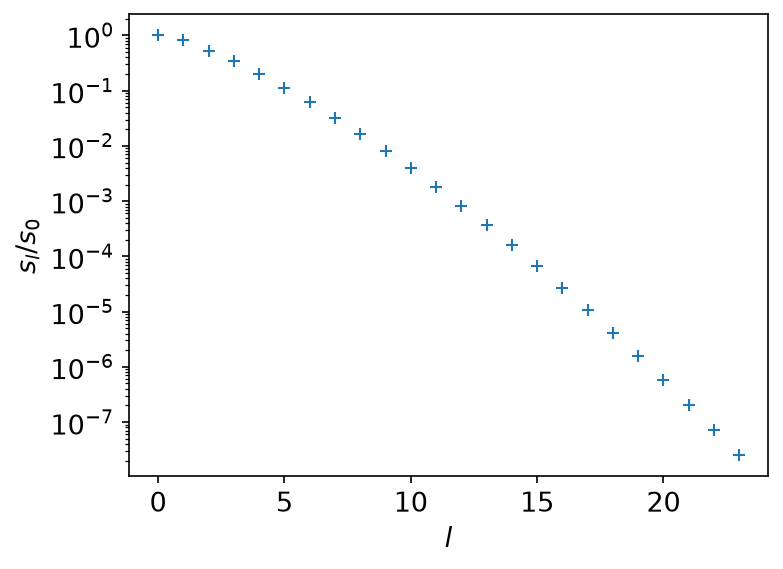
At \(\beta = 40\), \(\omega_\mathrm{max} = 2\) and \(\varepsilon = 2 \times 10^{-8}\) the basis has 24 functions and \(s_{23}/s_0 \approx 2.5 \times 10^{-8}\). Dividing by that last singular value multiplies whatever error rides on \(G_{23}\) by forty million. There is no algorithm that avoids this: the information about the fine structure of \(\rho\) is not in \(G\) to be recovered. All a method can do is choose what to put in its place.
Two models
Both are sums of normalised semicircles, so their exact \(\rho_l\) can be computed to machine precision and used as ground truth. One fills the band; the other is the same band split by a gap.
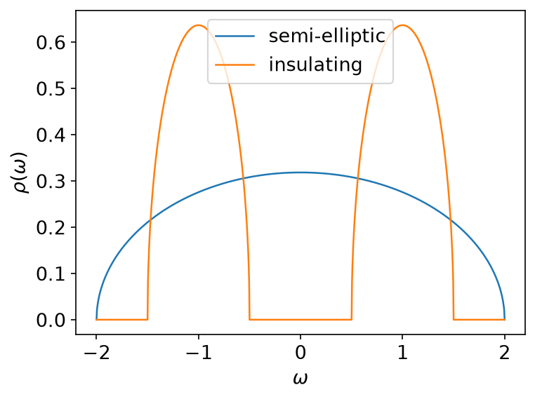
shifted_semicircle_overlaps (a tutorial helper) computes \(\rho_l\) of one
semicircle by quadrature, and \(G_l = -s_l \rho_l\):
    let rho_semi = shifted_semicircle_overlaps(&basis, 0.0, WMAX, 1.0);
    let rho_insul = {
        let right = shifted_semicircle_overlaps(&basis, WMAX / 2.0, WMAX / 4.0, 0.5);
        let left = shifted_semicircle_overlaps(&basis, -WMAX / 2.0, WMAX / 4.0, 0.5);
        right
            .iter()
            .zip(&left)
            .map(|(a, b)| a + b)
            .collect::<Vec<_>>()
    };
    let g_semi = coefficients(&s, &rho_semi);
    let g_insul = coefficients(&s, &rho_insul);
/// `Gₗ = −sₗ ρₗ`.
fn coefficients(s: &[f64], rho_l: &[f64]) -> Vec<f64> {
    s.iter().zip(rho_l).map(|(sl, rho)| -sl * rho).collect()
}
Then noise is added to \(G_l\), at \(0.3,(s_{L-1}/s_0)\) of \(\lVert G \rVert\) — deliberately of the same size as the smallest coefficient the basis still resolves.
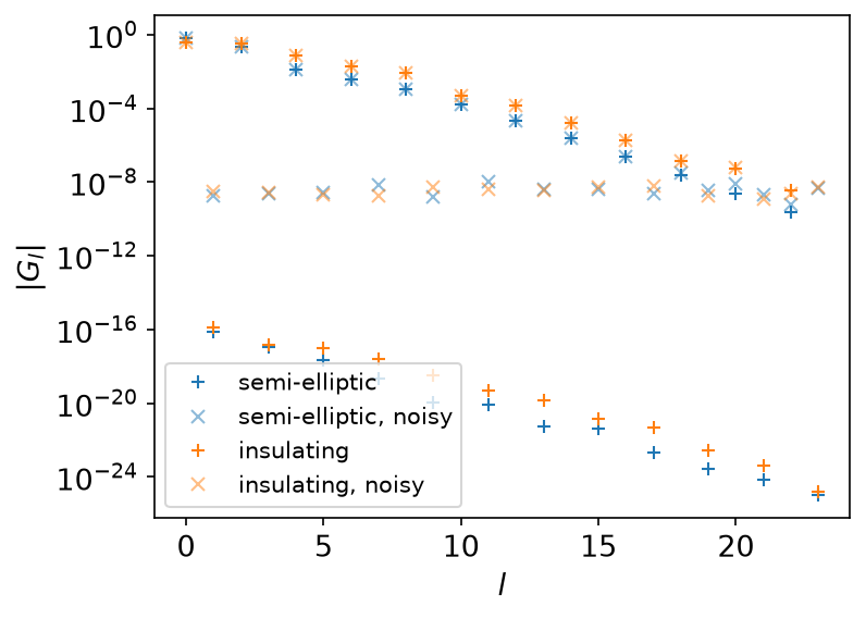
The noise is far below every coefficient that matters and level with the ones
at the end. The standard-normal draws are read from
docs/tutorial-code/input/analytic_continuation/noise.csv.
Truncated SVD
The first regulariser is the blunt one: keep \(\rho_l = -G_l/s_l\) for \(l < L’\) and throw the rest away.
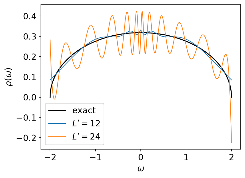
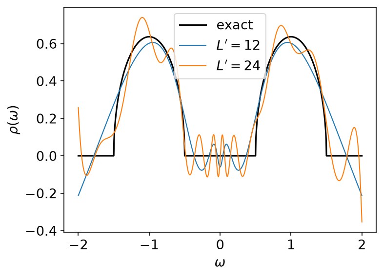
\(L’ = 12\) gets the shape right. \(L’ = 24\) — using everything the basis has — turns the answer into ringing of amplitude 0.2 around a function whose peak is 0.32. Using more of the data made the answer worse, which is the whole difficulty in one picture.
The insulating model says the same thing with a sharper edge:
Ridge regression
The second regulariser is smooth: minimise \(\lVert G - (-s\rho) \rVert^2 + \alpha^2 \lVert \rho \rVert^2\). Because the problem is diagonal in the basis, the solution is diagonal too,
\[ \rho_l = -\frac{s_l}{s_l^2 + \alpha^2}, G_l, \]
which passes the large singular values through unchanged and rolls the small ones off instead of dividing by them.
    let ridge: Vec<f64> = s.iter().map(|sl| -sl / (sl * sl + alpha * alpha)).collect();
    let rho_l_semi_ridge: Vec<f64> = ridge
        .iter()
        .zip(&g_semi_noisy)
        .map(|(r, g)| r * g)
        .collect();
    let rho_l_insul_ridge: Vec<f64> = ridge
        .iter()
        .zip(&g_insul_noisy)
        .map(|(r, g)| r * g)
        .collect();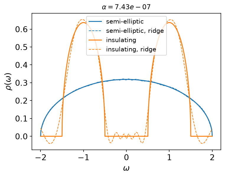
With \(\alpha = 100 \times \text{noise}\) both models come back recognisably. Note what is left over: the reconstruction goes negative inside the gap. A density of states cannot do that, and no amount of tuning \(\alpha\) will stop it, because nothing in the method knows that \(\rho \geq 0\).
Why ρl is the wrong unknown
It is tempting to conclude that the fix is a better penalty on \(\rho_l\). It is not, and the reason is worth stating plainly: \(G_l\) is compact, \(\rho_l\) is not. The basis is small because \(s_l\) makes it small — and \(s_l\) belongs to \(G\), not to \(\rho\).
Take four delta peaks, \(\rho(\omega) = \sum_i \delta(\omega - \omega_i)\), so that \(\rho_l = \sum_i v_l(\omega_i)\):
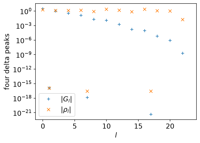
\(G_l\) falls off the way it always does. \(\rho_l\) does not fall off at all — it is still of order one at \(l = 23\), and would be at \(l = 200\). Truncating it at \(L’\) is not an approximation of anything; a penalty on \(\sum_l |\rho_l|^2\) is a penalty on coefficients that were never going to become small.
A spectrum made of a few poles is, on the other hand, exactly the case that pole-fitting methods handle well. MiniPole uses ESPRIT to fit a small number of poles and residues directly to Matsubara data, instead of expanding \(\rho\) in any basis.
A real-axis basis instead
So expand \(\rho\) on the real axis rather than in the IR basis:
\[ \rho(\omega) = \sum_{m} a_m, f(\omega - \omega_m), \qquad f(\omega) = \frac{1}{\pi}\frac{\eta}{\omega^2 + \eta^2}. \]
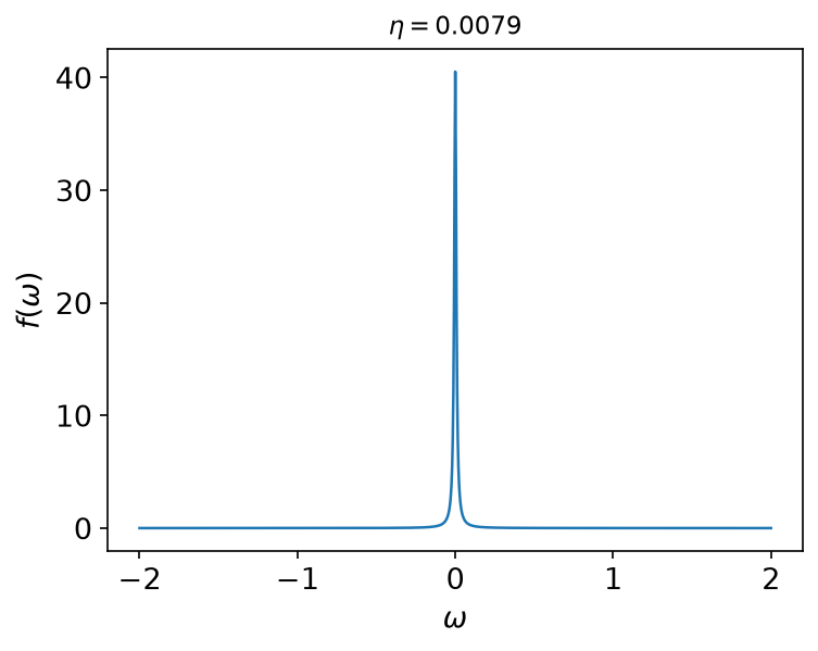
\(f\) is a probability density, so \(a_m \geq 0\) gives \(\rho \geq 0\) and \(\sum_m a_m = 1\) gives the sum rule — both of them constraints a solver can impose exactly, neither of them expressible in the IR coefficients. The width \(\eta\) is what is left to choose; \(\eta = 0.1,\pi/\beta\) is narrow enough to resolve structure on the scale of the temperature and wide enough not to be a set of delta functions.
The data then enter through
\[ G_l = \sum_m K_{lm} a_m, \qquad K_{lm} = -s_l \int \mathrm{d}\omega, v_l(\omega) f(\omega - \omega_m), \]
which is an ordinary constrained least-squares problem in \(a\).
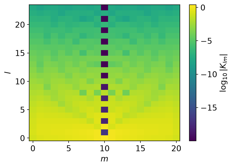
Computing \(K_{lm}\) is the one place this example does real numerical work. \(\eta\) is about a hundredth of the spacing between the basis’ knots, so quadrature on the knots steps straight over the peak of \(f\). The substitution \(\omega = \omega_m + \eta \tan t\) turns \(f(\omega - \omega_m),\mathrm{d}\omega\) into \(\mathrm{d}t/\pi\) and spreads the peak across the whole interval, leaving a polynomial to integrate:
/// `∫ dω vₗ(ω) f(ω − centre)` over the basis' ω range, to machine precision.
///
/// `η` is a small fraction of the knot spacing, so quadrature on the knots
/// alone would step straight over the peak. The substitution
/// `ω = centre + η tan t` turns `f(ω − centre) dω` into `dt/π` and spreads the
/// peak over the whole integration range; the knots come along as the segment
/// edges in `t`, where `vₗ` is still a polynomial in `ω`.
fn lorentz_overlaps(
    basis: &FiniteTempBasis<LogisticKernel, Fermionic>,
    centre: f64,
    eta: f64,
) -> Vec<f64> {
    let v = basis.v();
    let edges: Vec<f64> = v
        .get_knots(None)
        .into_iter()
        .map(|omega| ((omega - centre) / eta).atan())
        .collect();
    // tan t varies fast at the ends of each segment, so take more points than
    // the polynomial degree alone would need.
    let order = v.get_polyorder() + 24;

    (0..basis.size())
        .map(|l| {
            let poly = &v[l];
            integrate_segments(
                |t| poly.evaluate(centre + eta * t.tan()) / std::f64::consts::PI,
                &edges,
                order,
            )
        })
        .collect()
}
What this page stops short of
This page does not solve the constrained least-squares problem in \(a\). Sparse modeling solves a related one: an L1-regularised fit in the IR coefficients \(\rho_l\), without \(\rho \geq 0\) or the sum rule. Solving on the Lorentzian basis with both constraints imposed is the subject of the maximum-entropy and sparse-modeling literature, and is past where a tutorial ends.
Running it
From docs/tutorial-code:
$ cargo run --release --bin analytic_continuation
The program writes CSV tables to docs/tutorial-code/data/analytic_continuation/.
The figures are drawn from those tables; from the repository root, run
uv run --project docs/plotting python docs/plotting/analytic_continuation_plot.py.
The noise is committed rather than drawn at run time, so that this program and
its Python counterpart,
docs/tutorial-code/scripts/reference_analytic_continuation.py, use the same
numbers; the header of noise.csv says where the draws came from.
Key API pieces
From sparse-ir:
| What you want | What to call |
|---|---|
| the singular values | FiniteTempBasis::s |
| \(v_l\) on a grid of ω | Basis::evaluate_omega |
| the knots the basis is piecewise-polynomial on | basis.v().get_knots(None) |
| one \(v_l\) as a polynomial | basis.v()[l].evaluate(omega) |
| the degree to integrate exactly | basis.v().get_polyorder() |
From the tutorial crate (sparse_ir_tutorial, not part of the library):
| What you want | What to call |
|---|---|
| \(\rho_l\) of a semicircle | shifted_semicircle_overlaps |
| composite Gauss–Legendre quadrature over segments | integrate_segments |