MiniPole: a few complex poles from Matsubara data
sparse_ir::minipole is a Rust port of
Green-Phys/MiniPole (MIT License),
the reference implementation of the minimal pole method: L. Zhang and E. Gull,
Phys. Rev. B 110, 035154 (2024),
and, for matrix-valued functions, L. Zhang, Y. Yu and E. Gull,
Phys. Rev. B 110, 235131 (2024).
Both rest on the ESPRIT algorithm, available on its own as sparse_ir::esprit.
The Python tutorials have
no MiniPole notebook; this page is written for the Rust library.
MiniPole approximates a Green’s function by a small number of poles that are allowed to leave the real axis,
\[ G(z) \simeq C + \sum_{j} \frac{A_j}{z-\xi_j}. \]
The DLR uses a fixed grid of real poles \(\omega_p\) that works for every function with the same \(\beta\) and \(\omega_{\max}\). MiniPole instead adapts the poles \(\xi_j\) to one particular function. The result is much smaller than a DLR, it evaluates anywhere in the complex plane, and \(-\mathrm{Im}\,G(\omega+\mathrm{i}0)/\pi\) gives a spectral function, so it doubles as a tool for analytic continuation. A continuous spectrum is represented by poles pushed below the real axis.
What MiniPole gives you
Take the semicircular density of states \(\rho(\omega) = (2/\pi)\sqrt{1-\omega^2}\) on \([-1, 1]\). Its Green’s function \(G(z) = \int \mathrm{d}\omega\,\rho(\omega)/(z-\omega)\) is \(G(z) = 2\left(z - \sqrt{z-1}\sqrt{z+1}\right)\) on the physical sheet. With \(\beta=100\) and \(\omega_{\max}=1.5\), build a DLR, fit its coefficients to the exact \(G(\mathrm{i}\nu_n)\) at the DLR’s own sparse Matsubara nodes, and compress the coefficients with MiniPole:
use num_complex::Complex64;
use sparse_ir::minipole::{MiniPoleDlrParams, MiniPoleResult, mini_pole_dlr_from};
use sparse_ir::{
    Bosonic, DiscreteLehmannRepresentation, Fermionic, MatsubaraSampling, TypedTensor,
};
use std::error::Error;
use std::f64::consts::PI;
/// Semicircular DOS rho(w) = (2/pi) sqrt(1 - w^2) on [-1, 1]. Its Green's
/// function on the physical sheet is G(z) = 2 (z - sqrt(z-1) sqrt(z+1)).
fn semicircle(z: Complex64) -> Complex64 {
    2.0 * (z - (z - 1.0).sqrt() * (z + 1.0).sqrt())
}

/// Largest |G_MP(iv_n) - G(iv_n)| over the fermionic frequencies
/// iv_n = i n pi / beta with odd n, 0 < n < 2000. The poles lie in the lower
/// half plane, so G_MP represents G in the upper half plane only.
fn max_matsubara_error(rep: &MiniPoleResult, beta: f64) -> Result<f64, Box<dyn Error>> {
    let z: Vec<Complex64> = (0..1000)
        .map(|m| Complex64::new(0.0, (2 * m + 1) as f64 * PI / beta))
        .collect();
    let got = rep.evaluate(&z)?;
    Ok(got
        .host_data()?
        .iter()
        .zip(&z)
        .map(|(g, &zi)| (*g - semicircle(zi)).norm())
        .fold(0.0, f64::max))
}
    let (beta, wmax) = (100.0, 1.5);
    // An IR-independent DLR and its sparse Matsubara nodes.
    let dlr = DiscreteLehmannRepresentation::<Fermionic>::new(beta, wmax, 1e-12)?;
    let sampling = MatsubaraSampling::new(&dlr)?;
    let values: Vec<Complex64> = sampling
        .sampling_points()
        .iter()
        .map(|n| semicircle(n.value_imaginary(beta)))
        .collect();
    let values = TypedTensor::from_vec_col_major(vec![values.len()], values)?;
    let coeffs = sampling.fit_nd(None, &values, 0)?;

    // Contour from iw_5 = 11 pi / beta up to the default nmax = beta;
    // ESPRIT tolerance err = 1e-8.
    let rep = mini_pole_dlr_from(&dlr, &coeffs, &MiniPoleDlrParams::new(5, 1e-8))?;
    for pole in &rep.pole_location {
        println!("pole {:+.4} {:+.4}i", pole.re, pole.im);
        assert!(pole.im < 0.0, "pole {pole} is not in the lower half plane");
    }
    let error = max_matsubara_error(&rep, beta)?;
    println!(
        "{} poles (DLR size {}), max |G_MP - G| on iv_n = {error:.1e}",
        rep.pole_location.len(),
        dlr.poles().len()
    );
    assert!(error < 1e-3, "Matsubara error {error}");
Ok::<(), Box<dyn std::error::Error>>(())
The DLR has 39 poles. MiniPole returns five: \(\pm 0.940 - 0.151\mathrm{i}\), \(\pm 0.643 - 0.516\mathrm{i}\) and \(-0.737\mathrm{i}\). The code asserts that every pole lies in the lower half plane and that \(|G_{\rm MP}(\mathrm{i}\nu_n) - G(\mathrm{i}\nu_n)| < 10^{-3}\) for the positive fermionic frequencies \(\nu_n = n\pi/\beta\), \(n\) odd, \(n < 2000\); the actual maximum is \(1.8\times 10^{-4}\).
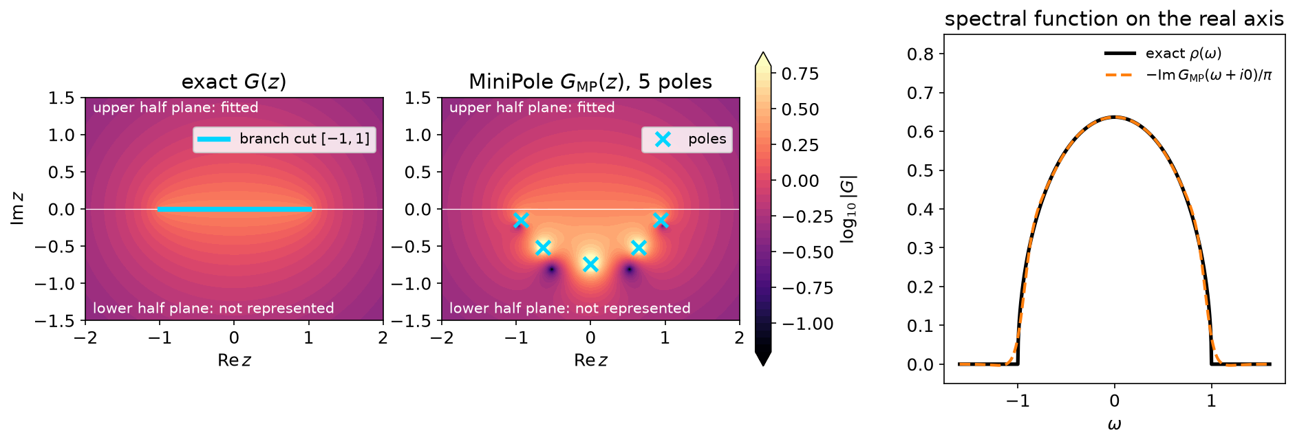
Left: \(\log_{10}|G(z)|\) of the exact function, analytic everywhere except on the branch cut \([-1,1]\). Middle: the MiniPole reconstruction. In the upper half plane, where the Matsubara data live, the two panels agree. The branch cut is replaced by five poles in the lower half plane; there, \(G_{\rm MP}\) is not meant to reproduce \(G\). Right: the spectral function \(-\mathrm{Im}\,G_{\rm MP}(\omega+\mathrm{i}0)/\pi\) against the exact semicircle. Since no pole is on or above the real axis, \(G_{\rm MP}(\omega+\mathrm{i}0)\) is simply \(G_{\rm MP}(\omega)\).
The number of poles is controlled by the ESPRIT tolerance err
(\(\varepsilon\) in the conventions).
It grows slowly as err decreases:
    // Fewer poles for a looser tolerance; err is not an error bound.
    let mut errs = Vec::new();
    let mut counts = Vec::new();
    let mut errors = Vec::new();
    for err in [1e-4, 1e-6, 1e-8, 1e-10] {
        let rep = mini_pole_dlr_from(&dlr, &coeffs, &MiniPoleDlrParams::new(5, err))?;
        assert!(rep.pole_location.iter().all(|p| p.im < 0.0));
        let error = max_matsubara_error(&rep, beta)?;
        println!(
            "err = {err:.0e}: {} poles, max error {error:.1e}",
            rep.pole_location.len()
        );
        errs.push(err);
        counts.push(rep.pole_location.len() as f64);
        errors.push(error);
    }
err | poles | max \(\lvert G_{\rm MP}-G\rvert\) on \(\mathrm{i}\nu_n\) |
|---|---|---|
| \(10^{-4}\) | 3 | \(7.4\times 10^{-3}\) |
| \(10^{-6}\) | 4 | \(1.2\times 10^{-3}\) |
| \(10^{-8}\) | 5 | \(1.8\times 10^{-4}\) |
| \(10^{-10}\) | 6 | \(3.0\times 10^{-5}\) |
err is a tolerance for the singular values inside ESPRIT. It is not a
bound on the error of \(G\): with err = 1e-8 the Matsubara error is
\(1.8\times 10^{-4}\).
Three entry points
| Function | Input | Frequencies | n0 means | Upper end of the contour |
|---|---|---|---|---|
mini_pole_dlr_from(&dlr, &coeffs, &p) | DLR coefficients \(g_l\) from MatsubaraSampling::fit_nd | contour \(\omega_n = (2n+1)\pi/\beta\), also for bosons | contour index | nmax (default \(\beta\)) |
mini_pole_dlr(&residues, &locations, beta, &p) | real poles and their actual residues | same as above | contour index | nmax |
mini_pole(&values, &freqs, &p) | \(G\) on a uniform, non-negative grid of physical frequencies \(\omega_n\) (real numbers, not indices) | as supplied | position in the array (N0::Auto by default) | last element |
C API spir_minipole_from_matsubara | as mini_pole | reduced indices \(n\), converted as \(\omega = n\pi/\beta\) | position in the array (\(<0\): automatic) | last element |
p is MiniPoleDlrParams for the first two and MiniPoleParams for
mini_pole. mini_pole_dlr_from forms the residues \(A_l = g_l w_l\) with
dlr.pole_weights() itself; bosonic DLR coefficients are not residues, so do
not pass them to mini_pole_dlr. The contour index of the DLR entry points is
not the reduced Matsubara index \(n\) used elsewhere in the library
(\(\mathrm{i}\nu_n = \mathrm{i}n\pi/\beta\)). The C function
spir_minipole_from_dlr follows mini_pole_dlr_from.
All of them return a MiniPoleResult with pole_location (\(\xi_j\), sorted
by real part), pole_weight (\(A_j\)), constant (\(C\)), and
evaluate(&z) for arbitrary complex \(z\). The full list of parameters
(symmetry, fixed pole count, N0::Auto, constant term, residue plane, C
arguments) is in the
sparse_ir::minipole module documentation.
Choosing the contour and err
MiniPole does not work on the Matsubara values directly. It maps the complex plane, cut along a segment of the imaginary axis, conformally onto the unit disk, so that the segment becomes the unit circle. It then computes moments of \(G\) along the segment and runs ESPRIT on those moments. For the DLR entry points the segment is
\[ [\mathrm{i}\omega_{n_0},\ \mathrm{i}\omega_{n_{\max}}],\qquad \omega_n=(2n+1)\pi/\beta . \]
n0sets the lower end. There is no automatic choice for DLR input.nmaxsets the upper end;Nonemeans \(n_{\max}=\beta\) (the number, in the units of the input). It is a floating-point cutoff, not a number of samples, and must exceedn0.erris the ESPRIT tolerance described above: set it at or above the noise level of the data.
The contour matters. Keep the same DLR coefficients and err = 1e-8, and
start the contour at three different points:
    // Same coefficients and err, three lower ends of the contour.
    let mut scan = Vec::new();
    for n0 in [0, 2, 5] {
        let rep = mini_pole_dlr_from(&dlr, &coeffs, &MiniPoleDlrParams::new(n0, 1e-8))?;
        let upper = rep.pole_location.iter().filter(|p| p.im > 0.0).count();
        let error = max_matsubara_error(&rep, beta)?;
        println!(
            "n0 = {n0}: {} poles, {upper} in the upper half plane, max error {error:.1e}",
            rep.pole_location.len()
        );
        scan.push((n0, upper, error, rep));
    }
    // n0 = 0 and 2 give spurious upper-half-plane poles; n0 = 5 does not.
    assert!(
        scan.iter()
            .all(|(n0, upper, ..)| (*n0 == 5) == (*upper == 0))
    );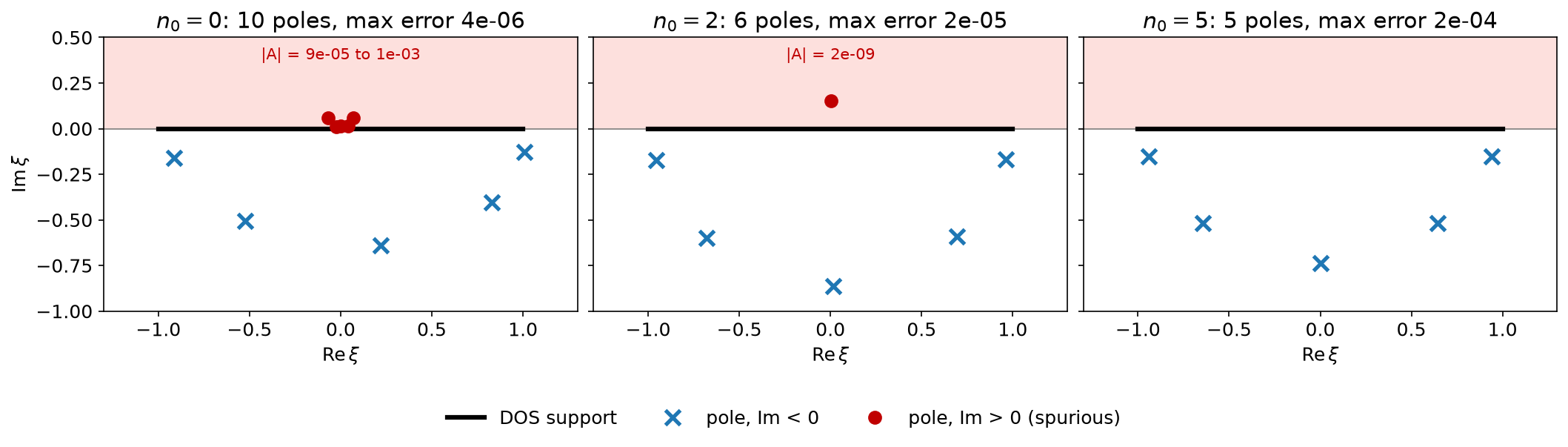
For n0 = 0 and n0 = 2 MiniPole returns extra poles in the upper half
plane, near the origin. Their weights are tiny (\(10^{-4}\) to
\(10^{-3}\) and \(2\times 10^{-9}\)), and the Matsubara error is in fact
smaller than for n0 = 5 (\(4\times10^{-6}\) and \(2\times10^{-5}\)
against \(2\times10^{-4}\)). But a pole with \(\mathrm{Im}\,\xi>0\) makes
\(G_{\rm MP}\) non-analytic in the upper half plane, so it cannot be a
retarded Green’s function. With n0 = 5 all poles are in the lower half plane.
The lesson: a small residual on the Matsubara axis does not validate the
contour; a pole in the upper half plane is the sign of a bad contour.
A harder case: a low-energy bosonic pair
Now take a bosonic susceptibility with \(\beta=20\), \(\omega_{\max}=3\), and the odd spectral function
\[ \rho(\omega)=\sum_j A_j\delta(\omega-\xi_j),\qquad (\xi_j,A_j)=(-1.2,-0.2),(-0.1,-0.3),(0.1,0.3),(1.2,0.2). \]
Thus \(\rho(-\omega)=-\rho(\omega)\), the inner pair has \(\beta|\xi|=2\), and \(\chi(0)=-19/3\) is finite. Fit the exact \(\chi(z)=\sum_j A_j/(z-\xi_j)\) at the DLR’s sparse Matsubara nodes and compress the coefficients. The DLR contour uses \((2n+1)\pi/\beta\) here too, even though the data are bosonic:
use num_complex::Complex64;
use sparse_ir::minipole::{MiniPoleDlrParams, MiniPoleResult, mini_pole_dlr_from};
use sparse_ir::{
Bosonic, DiscreteLehmannRepresentation, Fermionic, MatsubaraSampling, TypedTensor,
};
use std::error::Error;
use std::f64::consts::PI;
let (beta, wmax) = (20.0, 3.0);
// Odd spectral function: residues have opposite signs at +/- xi.
let spectrum = [(-1.2, -0.2), (-0.1, -0.3), (0.1, 0.3), (1.2, 0.2)];
let exact = |z: Complex64| -> Complex64 { spectrum.iter().map(|&(xi, a)| a / (z - xi)).sum() };
let dlr = DiscreteLehmannRepresentation::<Bosonic>::new(beta, wmax, 1e-12)?;
let sampling = MatsubaraSampling::new(&dlr)?;
let values: Vec<Complex64> = sampling
.sampling_points()
.iter()
.map(|n| exact(n.value_imaginary(beta)))
.collect();
let values = TypedTensor::from_vec_col_major(vec![values.len()], values)?;
let coeffs = sampling.fit_nd(None, &values, 0)?;
// These contour parameters resolve this particular low-energy pair.
let params = MiniPoleDlrParams {
nmax: Some(50.0),
..MiniPoleDlrParams::new(5, 1e-8)
};
let poles = mini_pole_dlr_from(&dlr, &coeffs, ¶ms)?;
assert_eq!(poles.pole_location.len(), 4);
// Independent analytic checks: pole and residue errors below 1e-3, and
// the static value chi(0) within 1 %.
for ((location, weight), &(xi, a)) in poles
.pole_location
.iter()
.zip(poles.pole_weight.host_data()?)
.zip(&spectrum)
{
assert!((*location - xi).norm() < 1e-3, "pole {xi}: {location}");
assert!((*weight - a).norm() < 1e-3, "residue {a}: {weight}");
}
let zero = Complex64::new(0.0, 0.0);
let chi0 = poles.evaluate(&[zero])?.host_data()?[0];
assert!((chi0 - exact(zero)).norm() < 1e-2 * exact(zero).norm());
Ok::<(), Box<dyn std::error::Error>>(())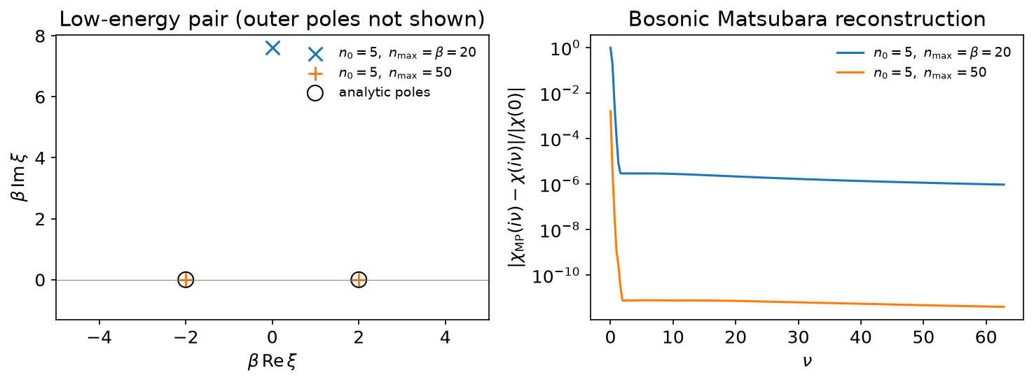
With n0 = 5, err = 1e-8 and the default nmax = beta = 20, MiniPole
returns three poles: the low-energy pair is merged into a single pole near
\(0.380\mathrm{i}\), again in the upper half plane. Extending the contour to
nmax = 50 gives four poles that match the exact ones to \(10^{-3}\), and
\(\chi_{\rm MP}(0)\) within 1 %. The left panel shows the inner poles (the
outer pair at \(\pm1.2\) is not shown); the right panel shows the error at
the bosonic frequencies \(\nu_m = 2m\pi/\beta\), including \(m=0\),
normalized by \(|\chi(0)|\).
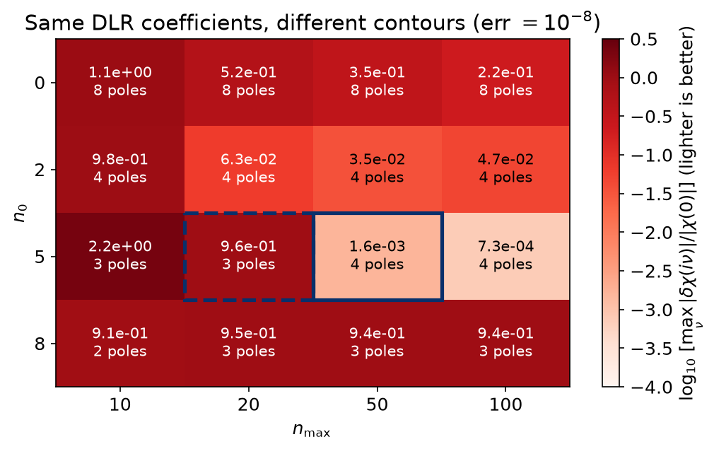
Each cell uses the same DLR coefficients and err = 1e-8. The number is
\(\max_{0\le m\le200}|\chi_{\rm MP}(\mathrm{i}\nu_m)-\chi(\mathrm{i}\nu_m)|/|\chi(0)|\)
and the second line the pole count; lighter cells are better. The dashed box
is the default contour, the solid box the one used above. Only n0 = 5 with
nmax = 50 or 100 brings the error below \(10^{-2}\). A longer contour is not a universal
cure, and neither n0 = 5 nor nmax = 50 is a general recommendation.
Practical checklist
- Compare a few contours (
n0,nmax) on the same data rather than trusting one. - Reject any result with a pole in the upper half plane.
- Check that the poles and residues are stable when the contour or
errchanges slightly. - Check the reconstruction at frequencies not used in the fit, especially near zero frequency.
- With noisy data, set
errat or above the noise level instead of asking for ever more poles.
A good fit at high Matsubara frequencies does not prove that a low-energy feature or the static response is right, and fitting imaginary frequencies does not guarantee a unique real-axis continuation for noisy data. The examples here have an exact answer to compare with; for measured data, stability and held-out residuals are diagnostics, not proof that the poles are physical.
Reproduce the figures
From docs/tutorial-code:
cargo run --profile ci --bin minipole
uv run --project ../plotting python ../plotting/minipole_plot.py
The binary writes CSV tables under docs/tutorial-code/data/minipole/; the
plotting script only reads them.