Discrete Lehmann representation
Ported from the Python notebook
DLR_py.ipynb
of the sparse-ir tutorials.
The program that produced every number and figure on this page is
docs/tutorial-code/src/bin/dlr.rs.
The discrete Lehmann representation (DLR) writes a Green’s function as a sum of poles on a fixed set of real frequencies \(\omega_p\):
\[ G(\mathrm{i}\nu) = \sum_{p} \frac{c_p, w_p}{\mathrm{i}\nu - \omega_p}, \qquad w_p = \begin{cases} 1 & \text{(fermions)},\ \tanh(\beta\omega_p/2) & \text{(bosons)}.\end{cases} \]
For fermions this is the spectral function
\(\rho(\omega) = \sum_p c_p, \delta(\omega - \omega_p)\) of delta peaks.
For bosons the logistic kernel expands \(\rho(\omega)/\tanh(\beta\omega/2)\)
rather than \(\rho(\omega)\) (see
Transformation from and to IR), and the
\(c_p\) are the weights of that function, so the residue of pole \(p\) is
\(c_p w_p\), not \(c_p\). DiscreteLehmannRepresentation::pole_weights()
returns the \(w_p\).
Like the IR basis, the DLR does not depend on the Green’s function: build it once for \(\beta\), \(\omega_\mathrm{max}\) and \(\varepsilon\), and expand any \(G\) in it.
There are two ways to choose the poles. The default,
DiscreteLehmannRepresentation::new(beta, wmax, eps), needs no IR basis. If
you already work with an IR basis, from_ir builds a DLR from it and gives you
the transform between the two sets of coefficients.
A DLR without an IR basis
DiscreteLehmannRepresentation::new picks the poles by an interpolative
decomposition (ID) of the logistic kernel, discretized on a fine grid of
\(\tau\) and \(\omega\): a column-pivoted Gram–Schmidt keeps adding poles
until the rest of the kernel lies within \(\varepsilon\) of their span. This
is the construction of Kaye, Chen and Parcollet, Phys. Rev. B 105,
235115 (2022). DlrBuilder does the same with a few more options, such as an
upper bound on the number of poles.
The model is the semicircle of the sparse sampling page,
\[ \rho(\omega) = \frac{2}{\pi}\sqrt{1-\omega^2}, \qquad G(\mathrm{i}\nu) = 2\mathrm{i}\left(\nu - \operatorname{sgn}(\nu)\sqrt{\nu^2+1}\right), \]
at \(\beta = 10^4\), \(\omega_\mathrm{max} = 1\) and \(\varepsilon = 10^{-14}\). The ID keeps 98 poles.
The DLR also chooses its own sampling points: as many Matsubara frequencies
(matsubara_nodes) and as many imaginary times (tau_nodes) as it has poles,
again by an ID. MatsubaraSampling::new(&dlr) and TauSampling::new(&dlr)
sample there, exactly as they sample at the default points of an IR basis. So
the whole workflow is: build, sample \(G\) at the nodes, fit.
    use num_complex::Complex64;
    use sparse_ir::{
        Basis, DiscreteLehmannRepresentation, Fermionic, FermionicFreq, MatsubaraSampling,
        TauSampling,
    };

    let (beta, wmax, eps) = (1e4, 1.0, 1e-14);
    // The poles come from an interpolative decomposition of the logistic
    // kernel; eps sets how many are kept.
    let dlr = DiscreteLehmannRepresentation::<Fermionic>::new(beta, wmax, eps)?;
    // The exact G(iν) of the semicircle at ν = nπ/β, written so that it does
    // not cancel at large |ν|.
    let g_exact = |nu: f64| Complex64::new(0.0, -2.0 * nu.signum() / (nu.abs() + nu.hypot(1.0)));

    // MatsubaraSampling::new samples at the DLR's own nodes,
    // dlr.matsubara_nodes(false): one frequency per pole.
    let sampling = MatsubaraSampling::<Fermionic>::new(&dlr)?;
    let g_iv: Vec<Complex64> = sampling
        .sampling_points()
        .iter()
        .map(|freq| g_exact(freq.value(beta)))
        .collect();
    // ρ is real, so ask for real coefficients.
    let c_p = sampling.fit_real(&g_iv)?;
Ok::<(), Box<dyn std::error::Error>>(())
The nodes are MatsubaraFreq values, so freq.value(beta) is
\(\nu_n = n\pi/\beta\) with the reduced index \(n\), odd for fermions (see
Conventions).
fit_real asks for real coefficients, which is right here because
\(\rho\) is real.
Once fitted, the DLR can be evaluated at any frequency. Here it is evaluated at odd \(n\) from 1 to about \(10^7\), far beyond the nodes, and compared with the closed form:
    // Evaluate the fitted DLR anywhere: here odd n from 1 to about 10⁷.
    let mut frequencies: Vec<i64> = (0..=140)
        .map(|k| (10f64.powf(k as f64 / 20.0).round() as i64) | 1)
        .collect();
    frequencies.dedup();
    let freqs: Vec<FermionicFreq> = frequencies
        .iter()
        .map(|&n| FermionicFreq::new(n))
        .collect::<Result<_, _>>()?;
    let dense = MatsubaraSampling::<Fermionic>::with_sampling_points(&dlr, freqs.clone())?;
    let g_iv_dlr = dense.evaluate_real(&c_p)?;
    let worst = freqs
        .iter()
        .zip(&g_iv_dlr)
        .map(|(freq, g)| (g - g_exact(freq.value(beta))).norm())
        .fold(0.0, f64::max);
    assert!(worst < 1e-12, "max |ΔG(iν)| = {worst:e}");
The imaginary-time nodes work the same way. There is no closed form for
\(G(\tau)\) of the semicircle, so the program takes \(G(\tau)\) at
tau_nodes from the first fit and fits the coefficients again from those
values alone. The sum rule \(G(0^+) + G(\beta^-) = -\int \rho = -1\) is an
independent check of the \(\tau\) side:
    // TauSampling::new samples at dlr.tau_nodes(). Fitting from G(τ) there
    // gives a DLR that is just as good on the Matsubara axis.
    let tau_sampling = TauSampling::<Fermionic>::new(&dlr)?;
    let g_tau = tau_sampling.evaluate(&c_p)?;
    let c_p_from_tau = tau_sampling.fit(&g_tau)?;
    let g_iv_from_tau = dense.evaluate_real(&c_p_from_tau)?;
    let worst_from_tau = freqs
        .iter()
        .zip(&g_iv_from_tau)
        .map(|(freq, g)| (g - g_exact(freq.value(beta))).norm())
        .fold(0.0, f64::max);
    assert!(worst_from_tau < 1e-11, "max |ΔG(iν)| = {worst_from_tau:e}");

    // G(0⁺) + G(β⁻) = −∫ρ(ω)dω = −1, a check that does not involve the fit
    // frequencies at all.
    let ends = dlr.evaluate_tau(&[0.0, beta])?;
    let sum_rule: f64 = (0..dlr.size())
        .map(|p| (ends.get(&[0, p]).unwrap() + ends.get(&[1, p]).unwrap()) * c_p[p])
        .sum();
    assert!((sum_rule + 1.0).abs() < 1e-11, "G(0) + G(β) = {sum_rule}");
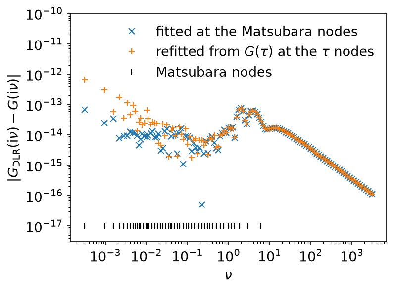
Both fits reproduce \(G(\mathrm{i}\nu)\) to better than \(10^{-12}\) on the whole axis (largest error \(7.6 \times 10^{-14}\) for the Matsubara fit, \(6.7 \times 10^{-13}\) for the fit from \(G(\tau)\)), and the sum rule holds to \(3.5 \times 10^{-13}\):
The coefficients themselves are not well determined: the condition numbers of these node matrices are large, and two fits can give different \(c_p\) that produce the same \(G\). Compare values of \(G\), not coefficients.
\(\varepsilon\) decides the number of poles, and asking for too much does
not pay. At \(\varepsilon = 10^{-15}\) the ID returns 192 poles instead of 98, the
node matrices become numerically singular (condition_number returns
infinity), and \(G(\mathrm{i}\nu)\) comes out less accurate, not more.
\(10^{-14}\) is about as small as \(\varepsilon\) usefully goes in double
precision, which is why the examples here pass it explicitly rather than
rely on the default.
A DLR from an IR basis
If your calculation already uses an IR basis, from_ir builds a DLR from it.
The poles are the roots of \(v_L(\omega)\), the first basis function the
truncation discarded, so there are exactly basis.size() of them, one per
basis function, whatever \(\varepsilon\) the basis was built with. This
choice is heuristic, but it makes the matrix \(v_l(\omega_p)\) well
conditioned, so that the IR and DLR coefficients convert into each other
without losing digits.
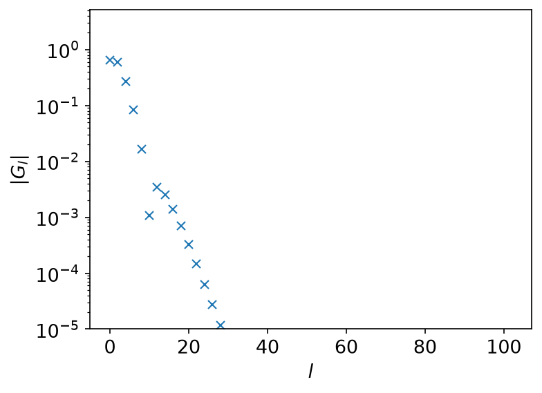
The model is the same semicircle at \(\Lambda = 10^4\), \(\omega_\mathrm{max} = 1\) and \(\varepsilon = 10^{-15}\): a basis of 104 functions, and therefore 104 poles. These are the exact IR coefficients \(g_l\):
    let kernel = LogisticKernel::new(BETA * WMAX)?;
    let basis = FiniteTempBasis::<LogisticKernel, Fermionic>::new(kernel, BETA, Some(EPS), None)?;
    // One pole per basis function, at the roots of the first discarded v_l.
    let dlr = DiscreteLehmannRepresentation::<Fermionic>::from_ir(&basis)?;
    let poles = dlr.poles().to_vec();
    assert_eq!(
        poles.len(),
        basis.size(),
        "an IR-derived DLR has one pole per basis function"
    );
An IR-derived DLR carries the transform to its source basis. from_ir_nd and
to_ir_nd are the two directions. They transform one axis of an array, so a
one-dimensional \(g_l\) goes in as a rank-1 tensor:
    // g_l -> c_p: one axis of a tensor, here a rank-1 tensor.
    let g_l_tensor = TypedTensor::from_vec_col_major(vec![basis.size()], g_l.clone())?;
    let c_p = dlr.from_ir_nd::<f64>(None, &g_l_tensor, 0)?;
    // c_p -> g_l
    let g_l_reconstructed = dlr.to_ir_nd::<f64>(None, &c_p, 0)?;
These two calls exist only on a DLR built by from_ir or
from_ir_with_poles. On a DLR built by new there is no IR basis to convert
to, and they return Error::NotSupported; use the DLR’s own nodes, as above.
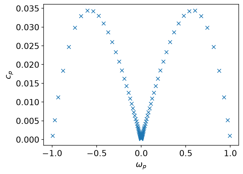
The coefficients sit on the poles like a sampled spectral function, which is what they are:
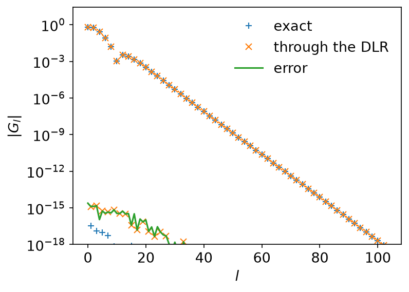
The round trip \(g_l \to c_p \to g_l\) costs nothing but rounding error:
Why bother
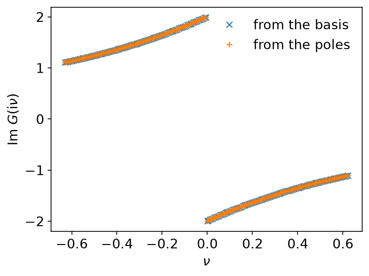
Because of what the poles let you do afterwards. The DLR is an analytic function of \(\mathrm{i}\nu\). Evaluating it anywhere is a sum over 104 terms, with no basis functions and no sampling matrix:
    // The DLR needs no basis functions here: it is a sum over poles,
    // G(iν) = Σ_p c_p w_p / (iν − ω_p). The weight w_p is 1 for fermions and
    // tanh(βω_p/2) for bosons.
    let weights = dlr.pole_weights();
    let g_iv_dlr: Vec<Complex64> = nu
        .iter()
        .map(|&nu| {
            (0..poles.len())
                .map(|p| {
                    *c_p.get(&[p]).unwrap() * weights[p] / (Complex64::new(0.0, nu) - poles[p])
                })
                .sum()
        })
        .collect();
For fermions \(w_p = 1\); written with pole_weights(), the same sum is
correct for bosons too. The answer agrees with the IR basis to the accuracy of
the basis, here out to \(|n| = 2000\), far beyond the sampling frequencies:
The same sum works for \(\tau\), for real frequencies just above the axis, and for products of Green’s functions, where the pole structure is what makes the convolution cheap.
Key API pieces
| What you want | What to call |
|---|---|
| a DLR without an IR basis (default) | DiscreteLehmannRepresentation::new(beta, wmax, eps), DlrBuilder |
| its sampling points | tau_nodes, matsubara_nodes; or TauSampling::new(&dlr), MatsubaraSampling::new(&dlr) |
| values → \(c_p\), \(c_p\) → values | fit, evaluate of either sampling object; MatsubaraSampling::fit_real, evaluate_real for real \(c_p\) |
| the default poles of an IR basis | DiscreteLehmannRepresentation::from_ir (trait DlrFromIr) |
| poles you chose yourself | DiscreteLehmannRepresentation::from_ir_with_poles |
| where the poles are | poles |
| the weights \(w_p\) | pole_weights |
| \(g_l \to c_p\), \(c_p \to g_l\) (IR-derived DLR only) | from_ir_nd, to_ir_nd |
A DiscreteLehmannRepresentation is itself a Basis, so evaluate_tau and
evaluate_matsubara work on it as they do on the IR basis.
Running it
From docs/tutorial-code:
cargo run --profile ci --bin dlr
uv run --project ../plotting python ../plotting/dlr_plot.py