Sparse sampling
Ported from the Python notebook
sparse_sampling_demo_py.ipynb
of the sparse-ir tutorials.
The program that produced every number and figure on this page is
docs/tutorial-code/src/bin/sparse_sampling_demo.rs.
This page shows how to infer the IR expansion coefficients of a Green’s function from its values at a handful of points. This is the sparse sampling technique that makes the basis useful in practice: you never need \(G\) on a dense grid, only at as many points as the basis has functions.
Setup
Take the semicircular spectral function of full bandwidth 2,
\[ \rho(\omega) = \frac{2}{\pi}\sqrt{1-\omega^2}, \]
at \(\beta = 10^4\) and \(\omega_\mathrm{max} = 1\). Asking for \(\varepsilon = 10^{-15}\) gives a basis of 104 functions.
use num_complex::Complex64;
use sparse_ir::{Fermionic, FiniteTempBasis, LogisticKernel, MatsubaraSampling, TauSampling};
/// Inverse temperature. Large enough that the basis is interesting (a few tens
/// of functions) while `ωmax = 1` keeps the spectral function simple.
const BETA: f64 = 10_000.0;
const WMAX: f64 = 1.0;
const EPS: f64 = 1e-15;
    let kernel = LogisticKernel::new(BETA * WMAX)?;
    let basis = FiniteTempBasis::<LogisticKernel, Fermionic>::new(kernel, BETA, Some(EPS), None)?;
Ok::<(), Box<dyn std::error::Error>>(())
The exact coefficients are \(g_l = -s_l \rho_l\) with \(\rho_l = \int \mathrm{d}\omega, v_l(\omega) \rho(\omega)\). They fall off exponentially, which is the whole reason the basis is small:
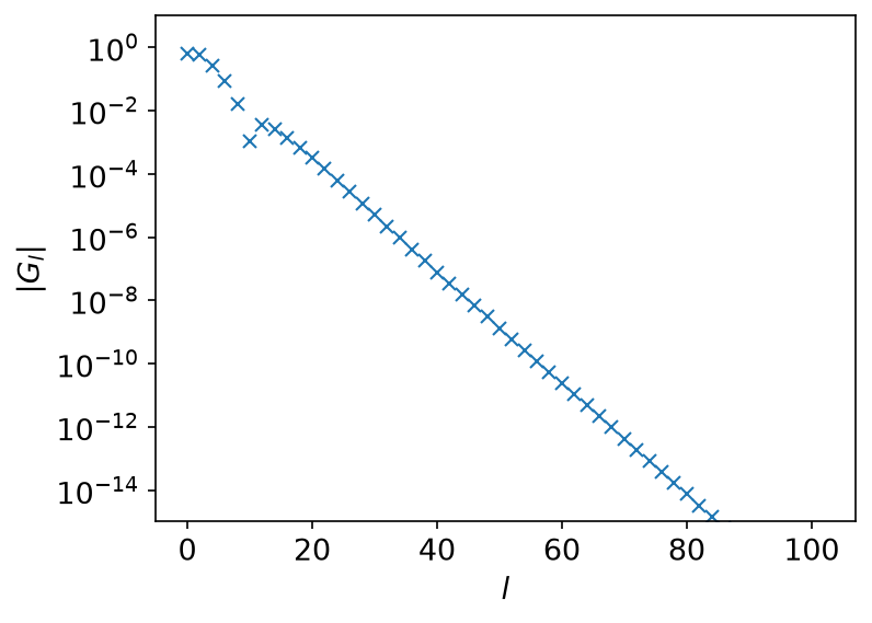
Only even \(l\) is shown: \(\rho\) is even in \(\omega\), so every odd coefficient vanishes.
From the sampling times
TauSampling picks the default sampling times, the roots of the first basis
function the truncation discarded, and builds the matrix
\(A_{il} = u_l(\tau_i)\) that turns coefficients into values. evaluate
goes from coefficients to values, fit the other way:
    let tau_sampling = TauSampling::<Fermionic>::new(&basis)?;
    let tau_points = tau_sampling.sampling_points().to_vec();
    // The default sampling times are folded around β/2, so they are reported
    // on the symmetric interval rather than on [0, β). See the conventions
    // page of the book.
    assert!(
        tau_points
            .iter()
            .all(|&tau| (-BETA / 2.0..=BETA / 2.0).contains(&tau)),
        "the default sampling times must lie in [-β/2, β/2]"
    );
    let g_tau = tau_sampling.evaluate(&g_l)?; // coefficients -> values
    let g_l_from_tau = tau_sampling.fit(&g_tau)?; // values -> coefficients
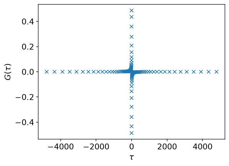
There are 104 sampling times, as many as the basis has functions, and the
condition number (condition_number) is about 51.8. A fit from the sampling
times therefore loses one or two significant digits, no more.
The times come back on \([-\beta/2, \beta/2]\) rather than on \([0, \beta)\); see Conventions for why.
From the sampling frequencies
MatsubaraSampling does the same in frequency. Its points are MatsubaraFreq
values, and n() returns the reduced index \(n\) of
\(\mathrm{i}\nu_n = \mathrm{i}n\pi/\beta\). For fermions \(n\) is odd
(\(n = 2m + 1\) in terms of the textbook index \(m\)), so
FermionicFreq::new(1) is \(\nu = \pi/\beta\) and FermionicFreq::new(0) is
an error; see
Conventions.
\(G\) is complex there, so the coefficients go in and come back as
Complex64:
    let matsubara_sampling = MatsubaraSampling::<Fermionic>::new(&basis)?;
    // The points are MatsubaraFreq values; n() is the reduced index n of
    // iν_n = i n π/β, which is odd for fermions.
    let matsubara_points: Vec<i64> = matsubara_sampling
        .sampling_points()
        .iter()
        .map(|freq| freq.n())
        .collect();
    assert!(
        matsubara_points.iter().all(|n| n % 2 != 0),
        "fermionic Matsubara indices must be odd"
    );
    // G(iν) is complex, so the coefficients go in, and come back, as Complex64.
    let g_l_complex: Vec<Complex64> = g_l.iter().map(|&g| Complex64::new(g, 0.0)).collect();
    let g_iv = matsubara_sampling.evaluate(&g_l_complex)?;
    let g_l_from_matsubara: Vec<f64> = matsubara_sampling
        .fit(&g_iv)?
        .iter()
        .map(|c| c.re)
        .collect();
The coefficients here are real, so the complex copy is not needed:
evaluate_real takes real coefficients and returns complex values, and
fit_real fits real coefficients to complex values.
The condition number is about 213, roughly four times that of the sampling times. That is the price of working in frequency.
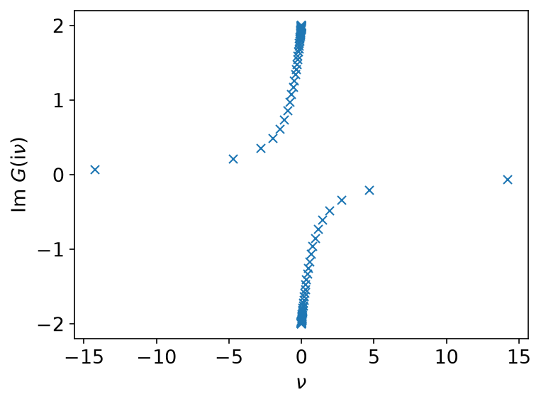
Because \(\rho\) is even in \(\omega\), \(G(\mathrm{i}\nu)\) is purely imaginary; the real part that comes back is rounding error, about \(10^{-15}\) of the imaginary part.
Comparison with the exact result
Both fits recover the exact coefficients:
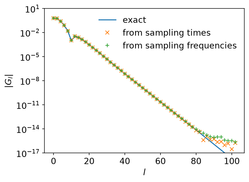
The curves lie on top of each other until the coefficients themselves drop below \(10^{-14}\), where there is nothing left to recover. The differences say the same thing more directly:
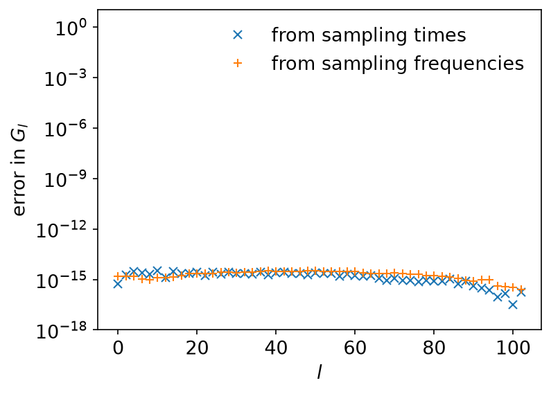
The error sits at \(10^{-16}\)–\(10^{-15}\). The accuracy of the basis times the condition number of the fit bounds it by about \(10^{-15} \times 52 \approx 5 \times 10^{-14}\) from the sampling times and \(10^{-15} \times 213 \approx 2 \times 10^{-13}\) from the sampling frequencies, so both fits are well within the bound.
Key API pieces
| What you want | What to call |
|---|---|
| the sampling points | TauSampling::sampling_points, MatsubaraSampling::sampling_points |
| the reduced index of a Matsubara point | MatsubaraFreq::n |
| how much a fit costs you | condition_number |
| coefficients → values | evaluate (evaluate_real for real coefficients in frequency) |
| values → coefficients | fit (fit_real for real coefficients in frequency) |
| your own points instead of the defaults | TauSampling::with_sampling_points, MatsubaraSampling::with_sampling_points |
evaluate and fit have _to variants that write into a slice you own, and
_nd variants for a whole array of Green’s functions sharing one basis. Use
those in an inner loop, where allocating per call would dominate.
The same sampling objects work on a DLR: TauSampling::new(&dlr) and
MatsubaraSampling::new(&dlr) sample at the DLR’s own nodes. See
Discrete Lehmann representation.
Running it
From docs/tutorial-code:
cargo run --profile ci --bin sparse_sampling_demo
uv run --project ../plotting python ../plotting/sparse_sampling_demo_plot.py