Transformation from and to IR
Ported from the Python notebook
transformation_py.ipynb
of the sparse-ir tutorials.
The program that produced every number and figure on this
page is docs/tutorial-code/src/bin/transformation.rs.
The basis is only useful once your data is in it. This page covers the three ways data usually arrives (as poles, as a smooth spectral function, as \(G(\tau)\) on a grid) and the way back out.
Poles
A Green’s function made of poles,
\[ G(\mathrm{i}\nu) = \sum_{p} \frac{a_p}{\mathrm{i}\nu - \omega_p}, \qquad A(\omega) = \sum_p a_p \delta(\omega - \omega_p), \]
needs no quadrature at all. The logistic kernel expands the regularized spectral function, which for bosons carries an extra factor,
\[ \rho(\omega) = \sum_p c_p \delta(\omega - \omega_p), \qquad c_p = \begin{cases} a_p & \text{(fermions)},\ a_p / \tanh(\beta\omega_p/2) & \text{(bosons)},\end{cases} \]
so the overlap integral collapses to \(\rho_l = \sum_p c_p v_l(\omega_p)\).
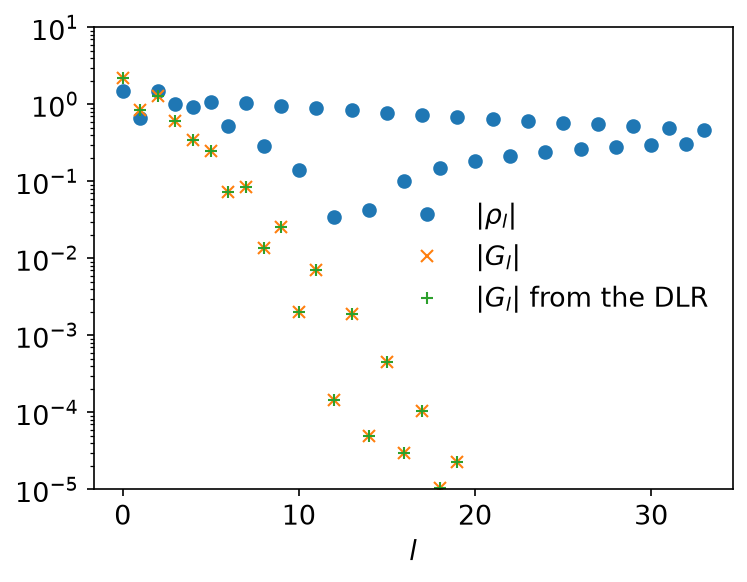
The example takes one bosonic pole at \(\omega_1 = 0.1\) with
\(a_1 = 1\), at \(\beta = 15\), \(\omega_\mathrm{max} = 10\) and
\(\varepsilon = 10^{-10}\), a basis of 34 functions. evaluate_omega
gives the \(v_l(\omega_p)\), and \(g_l = -s_l \rho_l\). The
DiscreteLehmannRepresentation says the same thing in one call: build it with
the poles (from_ir_with_poles), and to_ir_nd turns the DLR coefficients
\(c_p\) into IR coefficients (see
Discrete Lehmann representation).
use std::error::Error;

use sparse_ir::DlrFromIr;
use sparse_ir::{
    Basis, Bosonic, DiscreteLehmannRepresentation, Fermionic, FiniteTempBasis, LogisticKernel,
    MatsubaraSampling, TauSampling,
};
use sparse_ir::{Matrix, TypedTensor};
/// The pole section: one bosonic pole, placed just off zero so that the
/// `1/tanh(βω/2)` regularizer is large but finite.
const POLE_BETA: f64 = 15.0;
const POLE_WMAX: f64 = 10.0;
const POLE_EPS: f64 = 1e-10;
const POLE_POSITION: f64 = 0.1;
const POLE_WEIGHT: f64 = 1.0;
fn pole_basis() -> Result<FiniteTempBasis<LogisticKernel, Bosonic>, Box<dyn Error>> {
    let kernel = LogisticKernel::new(POLE_BETA * POLE_WMAX)?;
    Ok(FiniteTempBasis::<LogisticKernel, Bosonic>::new(
        kernel,
        POLE_BETA,
        Some(POLE_EPS),
        None,
    )?)
}
    let basis = pole_basis()?;

    // For the logistic kernel the bosonic spectral function carries the
    // `1/tanh(βωₚ/2)` factor, so that is what the basis expands.
    let regularized = POLE_WEIGHT / (0.5 * POLE_BETA * POLE_POSITION).tanh();

    let v_at_pole: Matrix<f64> = basis.evaluate_omega(&[POLE_POSITION])?;
    let rho_l: Vec<f64> = (0..basis.size())
        .map(|l| *v_at_pole.get(&[0, l]).unwrap() * regularized)
        .collect();
    let g_l: Vec<f64> = basis
        .s()
        .iter()
        .zip(&rho_l)
        .map(|(s, rho)| -s * rho)
        .collect();

    // The DLR says the same thing in one call: it knows how a pole maps onto
    // the basis, so it takes the DLR coefficient `cₚ = aₚ/tanh(βωₚ/2)` and
    // returns `gₗ` directly.
    let dlr =
        DiscreteLehmannRepresentation::<Bosonic>::from_ir_with_poles(&basis, vec![POLE_POSITION])?;
    let weights = TypedTensor::from_vec_col_major(vec![1], vec![regularized])?;
    let g_l_dlr = dlr.to_ir_nd::<f64>(None, &weights, 0)?;
Ok::<(), Box<dyn std::error::Error>>(())
Both routes give the same coefficients:
From a smooth spectral function
For a smooth \(\rho\) the coefficients are an integral,
\[ \rho_l = \int_{-\omega_\mathrm{max}}^{\omega_\mathrm{max}} \mathrm{d}\omega, v_l(\omega), \rho(\omega). \]
A single Gauss-Legendre rule over the whole interval will not do. The roots of \(v_l\) crowd together near \(\omega = 0\), far more densely than the roots of a Legendre polynomial of the same degree, so the integrand varies on a scale the rule cannot see. Split the interval at the knots the basis functions are built on, where each \(v_l\) is a polynomial, and apply the rule on every piece; if \(\rho\) is smooth within a piece, the result converges exponentially in the order.
PiecewiseLegendrePolyVector::get_knots hands you exactly those division
points. integrate_segments is a tutorial-crate helper that applies a
Gauss-Legendre rule on every segment; sparse_ir::legendre provides such a
rule if you want to write your own.
fn overlap_with_v<F>(basis: &FiniteTempBasis<LogisticKernel, Fermionic>, f: F) -> Vec<f64>
where
    F: Fn(f64) -> f64,
{
    let v = basis.v();
    let edges = v.get_knots(None);
    let order = v.get_polyorder() + 8;
    (0..basis.size())
        .map(|l| {
            let poly = &v[l];
            integrate_segments(|omega| poly.evaluate(omega) * f(omega), &edges, order)
        })
        .collect()
}
With \(\rho_l\) in hand, \(g_l = -s_l \rho_l\).
The spectral function here is three Gaussian peaks, one of them narrow:
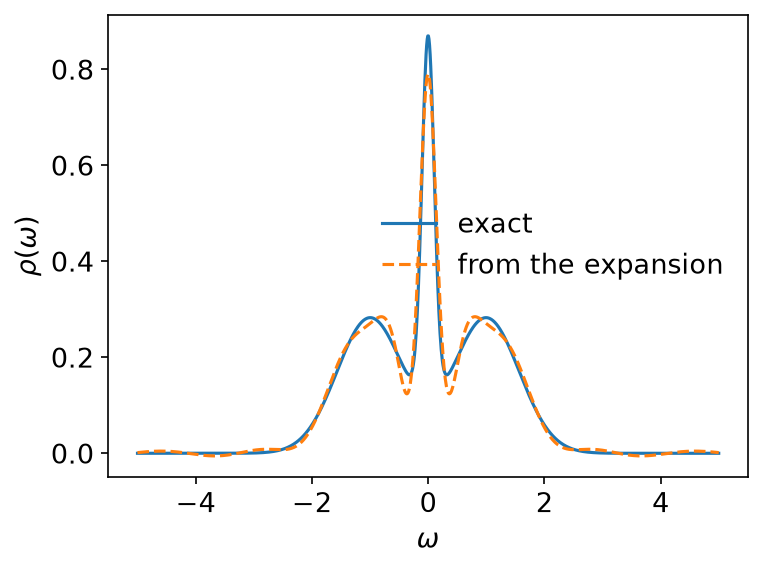
The dashed line is \(\sum_l v_l(\omega) \rho_l\), evaluated on a grid the basis never saw: the expansion is good everywhere, not only at the knots.
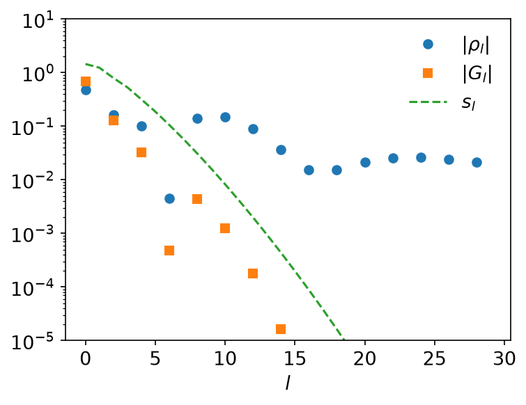
\(g_l\) falls off like \(s_l\); \(\rho_l\) does not, because the narrow peak needs high \(l\) to resolve. That is the normal picture, and the next section shows what the abnormal one looks like.
From IR to imaginary time
With \(g_l\) in hand, \(G(\tau) = \sum_l u_l(\tau) g_l\) on any grid you
like. Either evaluate the basis functions (evaluate_tau returns a
[taus.len(), basis.size()] matrix),
    // Directly: `G(τ) = Σₗ uₗ(τ) gₗ`.
    let u_at_taus: Matrix<f64> = basis.evaluate_tau(&taus)?;
    let g_tau_direct: Vec<f64> = (0..taus.len())
        .map(|i| {
            (0..basis.size())
                .map(|l| *u_at_taus.get(&[i, l]).unwrap() * g_l[l])
                .sum()
        })
        .collect();
or hand the same points to TauSampling, which builds that matrix once and
can also go back the other way:
    // Or through `TauSampling`, which builds the same matrix once and can also
    // go the other way. Any set of τ points will do — these are not the
    // default sampling times.
    let sampling = TauSampling::<Fermionic>::with_sampling_points(basis, taus.clone())?;
    let g_tau_sampling = sampling.evaluate(&g_l)?;
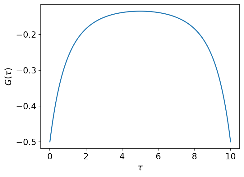
Nothing requires these to be the default sampling points. They are an arbitrary dense grid here, which is what you want for a figure:
From full imaginary-time data
Going back from \(G(\tau)\) known everywhere, the stable route is the overlap integral
\[ g_l = \int_0^\beta \mathrm{d}\tau, G(\tau), u_l(\tau), \]
by the same composite quadrature as before, now on the knots of basis.u().
It recovers the coefficients to the accuracy of the basis:
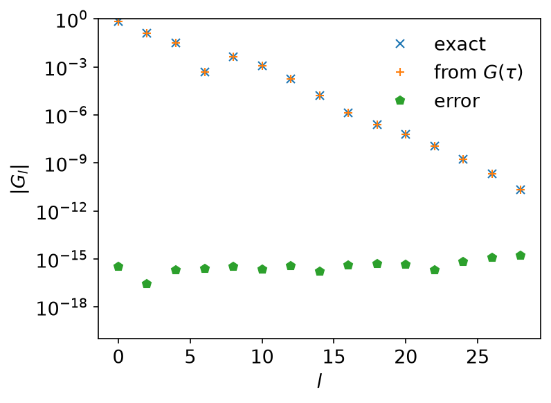
Only even \(l\) is shown: \(\rho\) is even in \(\omega\), so the odd coefficients vanish.
What if ωmax is too small?
Expand the very same \(G(\tau)\) in a basis built for \(\omega_\mathrm{max} = 0.5\), far too narrow for a spectral function that reaches out to \(\omega \approx 3\):
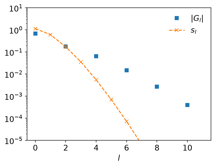
The coefficients stop following the singular values down. That is the signal, and the only one you get: nothing errors, the expansion simply does not converge. If \(g_l\) does not decay like \(s_l\), widen \(\omega_\mathrm{max}\).
Many Green’s functions at once
evaluate and fit have _nd variants that transform one axis of an array,
which is what you want when many Green’s functions share a basis: orbital
indices, momenta, a self-energy on a grid.
    // coeffs has shape [2, 3, basis.size()]; transform along axis 2.
    let sampling = MatsubaraSampling::<Fermionic>::new(basis)?;
    let values = sampling.evaluate_nd_real(None, &coeffs, 2)?;
    let recovered = sampling.fit_nd_real(None, &values, 2)?;
The _real variants take real coefficients and return complex values, which
saves you building a complex copy of an array that has no imaginary part.
Key API pieces
| What you want | What to call |
|---|---|
| \(v_l\) or \(u_l\) at your own points | Basis::evaluate_omega, Basis::evaluate_tau |
| the segments to integrate over | PiecewiseLegendrePolyVector::get_knots |
| a Gauss-Legendre rule | sparse_ir::legendre |
| DLR coefficients \(c_p\) → \(g_l\) | DiscreteLehmannRepresentation::from_ir_with_poles, to_ir_nd |
| one axis of an array | the _nd and _nd_real variants |
Tutorial-crate helper (not part of sparse-ir):
| What you want | What to call |
|---|---|
| a composite Gauss-Legendre integral over given segments | sparse_ir_tutorial::integrate_segments |
Running it
From docs/tutorial-code:
cargo run --profile ci --bin transformation
uv run --project ../plotting python ../plotting/transformation_plot.py