Exchange interactions
Ported from the Python notebook
liechtenstein_py.ipynb
of sparse-ir-tutorial,
whose author is Takuya Nomoto. The program that produced every number and
figure on this page is docs/tutorial-code/src/bin/liechtenstein.rs; the code
below is included from it.
Both previous applied pages used the basis to hold a function of imaginary time. This one uses it for something narrower and, in its way, more striking: to do a Matsubara sum in one evaluation.
Theory
The Liechtenstein method reads the parameters of a classical spin model off an itinerant one by requiring that the two have the same second derivative of the total energy with respect to spin angles. For a single orbital,
\[ H = -t \sum_{\langle i, j\rangle, s} c^\dagger_{is} c_{js}
- \sum_i \sum_{ss’} c^\dagger_{is} (\boldsymbol{B}i \cdot \boldsymbol{\sigma}{ss’}) c_{is’}, \]
expanded about the ferromagnetic state \(\boldsymbol{B}_i = B\hat{z}\), the requirement gives
\[ J_{ij} = -B^2 T \sum_\nu G_{ij,+}(\mathrm{i}\nu) G_{ji,-}(\mathrm{i}\nu), \]
and, for the quantity that sets the mean-field transition temperature \(T_c^\mathrm{mf} = 2J_0/3\),
\[ J_0 = \frac{B}{2}(n_{0,+} - n_{0,-}) + B^2 T \sum_\nu G_{00,+}(\mathrm{i}\nu) G_{00,-}(\mathrm{i}\nu). \]
Here \(G_{ij,\pm}\) is the Green’s function of spin \(\pm\) in the field, and \(\nu = \nu_n = n\pi/\beta\) runs over all fermionic frequencies (\(n\) odd). Both are Matsubara sums of a product of two Green’s functions. That product falls off as \(1/\nu^2\), so a truncated sum converges like \(1/N_M\) — slowly, and the more slowly the colder the system.
Parameters
The example uses a square lattice with nearest-neighbour hopping \(t = 1\) on a \(36 \times 36\) momentum grid, the field \(B = 3\), \(\beta = 50\) and \(\varepsilon = 10^{-7}\). \(J_0\) is scanned over 41 chemical potentials from \(\mu = -10\) to \(10\); \(J_{ij}\) is computed at half filling, \(\mu = 0\). The basis has to hold both spin-split bands, so \(\omega_\mathrm{max} = 2 \max(W, B) = 16\) with the bandwidth \(W = 8t\), and \(\Lambda = \beta\omega_\mathrm{max} = 800\).
const T_HOPPING: f64 = 1.0;
const BETA: f64 = 50.0;
const NK_LIN: usize = 36;
/// The effective field that polarizes the reference state.
const B_EFF: f64 = 3.0;
const EPS: f64 = 1e-7;
/// `2 max(W, B) β` with the bandwidth `W = 8t`: the basis has to hold the
/// whole of both spin-split bands.
const LAMBDA: f64 = 2.0 * 8.0 * T_HOPPING * BETA;
/// How many chemical potentials `J₀` is scanned over, from −10 to 10.
const N_MU: usize = 41;
/// The truncated Matsubara grids `J₀` is also evaluated on, for comparison.
const NAIVE: [usize; 5] = [100, 200, 400, 800, 1600];
The sum as an evaluation
The way out is the elementary identity
\[ T \sum_\nu F(\mathrm{i}\nu) = F(\tau = 0), \]
which turns the sum into one point of the imaginary-time function behind it. A product of two Green’s functions is as representable in the basis as a single one, so the whole sum costs a fit and one evaluation:
    // `T Σ_ν F(iν) = F(τ = 0)`: the Matsubara sum is the basis expansion read
    // at one point. This is the row of basis functions that reads it.
    let u_at_zero = basis.evaluate_tau(&[0.0])?;
    let occupation = occupation_term(&ek, &mu);
    // One column per chemical potential, one row per sampling frequency.
    let mut sampled = Vec::with_capacity(mesh.n_wn() * N_MU);
    for freq in mesh.wn() {
        sampled.extend(product_at(freq.value(BETA), &ek, &mu));
    }
    let coefficients = mesh.wn_to_l(&sampled, N_MU)?;
    let summed = evaluate_rows(&u_at_zero, &coefficients, N_MU);
    let j0: Vec<f64> = occupation
        .iter()
        .zip(&summed)
        .map(|(n, s)| n + s.re)
        .collect();
sampled holds the product at the 38 sampling frequencies, one column per
chemical potential; evaluate_rows (a tutorial helper) contracts the
coefficients with \(u_l(0)\). At \(\beta = 50\) and \(\Lambda = 800\)
the basis has 37 functions. The size grows only like \(\log \beta\): since
\(\Lambda = 16t\beta\) here, \(\beta = 500\) gives 53 functions and
\(\beta = 5000\) gives 68, for a hundred times lower temperature.
The example also sums the series the naive way, on symmetric grids of 200 to 3200 frequencies (100 to 1600 on each side of zero), so that the two can be put side by side:
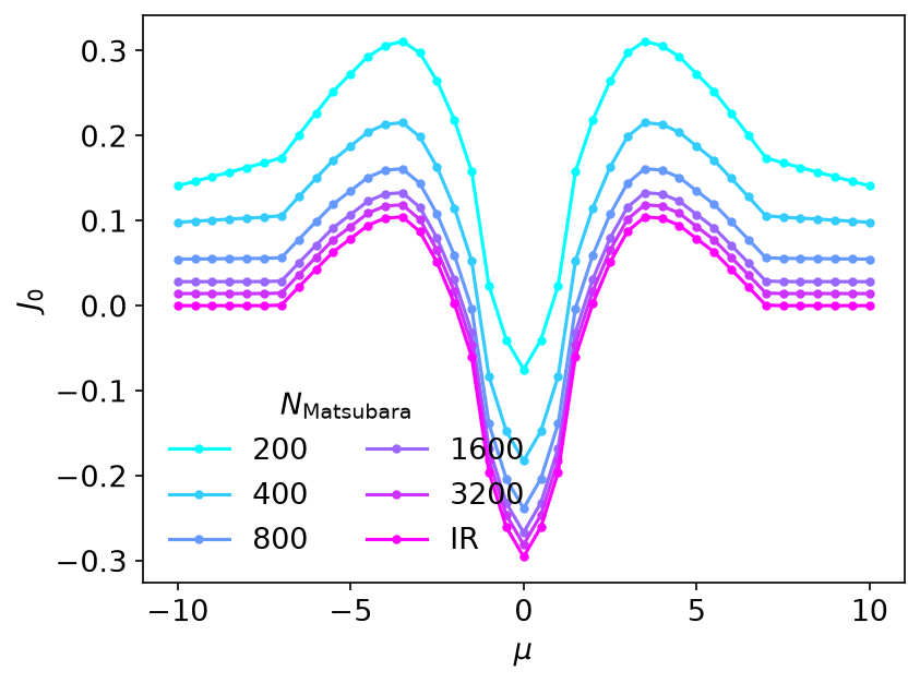
The truncated sums are above the converged answer everywhere and creep down towards it. How fast is the whole story:
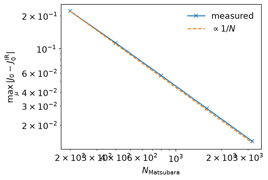
Halving the error costs a doubling of the grid. Reaching the basis answer that way would take of order \(10^{9}\) frequencies; the basis reaches it with 38.
The physics, once the answer is trusted: \(J_0 < 0\) at half filling, where the system is an antiferromagnet by super-exchange, and \(J_0 > 0\) in the low-carrier regime, where double exchange makes it a ferromagnet.
\(J_{ij}\), and a check
\(J_{ij}\) needs the Green’s function in real space rather than its zone average, so a Fourier transform joins the sum. \(G_{ij}\) carries \(e^{-\mathrm{i}k\cdot r}\) and \(G_{ji}\) carries \(e^{+\mathrm{i}k\cdot r}\); since \(\epsilon_{\boldsymbol{k}}\) is even, the second is the first applied to the same array. The program checks that before relying on it:
    assert!(
        (0..grid.len()).all(|index| {
            let (k1, k2) = (index / NK_LIN, index % NK_LIN);
            let mirrored = ((NK_LIN - k1) % NK_LIN) * NK_LIN + (NK_LIN - k2) % NK_LIN;
            (ek[index] - ek[mirrored]).abs() < 1e-12
        }),
        "the dispersion must be even in k for G_ji to be the transform of G_ij"
    );
The on-site term \(J_{00}\) is not an exchange interaction, so it is set to zero:
    // The on-site term is not an exchange interaction; the notebook drops it.
    jij[0] = 0.0;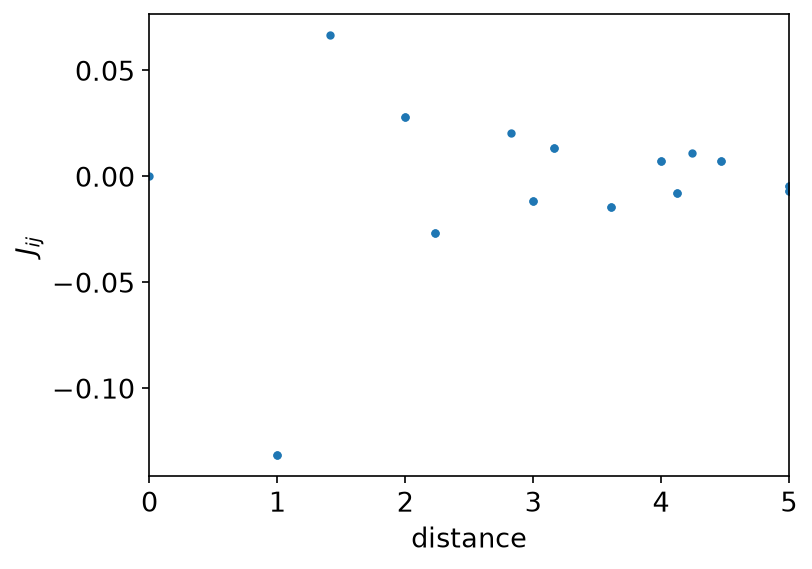
The sum rule \(J_0 = \sum_{j \ne 0} J_{0j}\) then connects the two calculations, which took different routes: one never left momentum space, the other summed the 1295 off-site terms of the \(36 \times 36\) real-space lattice. At \(\mu = 0\) they agree to \(4 \times 10^{-8}\) (\(J_0 \approx -0.2954590\)), which is the accuracy of the basis (\(\varepsilon = 10^{-7}\)) and not machine precision — as it should be.
Going further
This page uses only the IR basis and stays on the imaginary axis. For real-frequency output, see MiniPole, which fits a few poles to Matsubara data by ESPRIT, and Analytic continuation for why that step is ill posed. The DLR page shows the pole-based representation of imaginary-axis data.
Running it
From docs/tutorial-code:
$ cargo run --release --bin liechtenstein
The program writes CSV tables to docs/tutorial-code/data/liechtenstein/. The
figures are drawn from those tables; from the repository root, run
uv run --project docs/plotting python docs/plotting/liechtenstein_plot.py.
Key API pieces
From sparse-ir:
| What you want | What to call |
|---|---|
| a Matsubara sum | fit (MatsubaraSampling::fit_nd), then evaluate at τ = 0 |
| the row \(u_l(0)\) | Basis::evaluate_tau(&[0.0]) |
From the tutorial crate (sparse_ir_tutorial, not part of the library):
| What you want | What to call |
|---|---|
| many chemical potentials at once | one column each; IrMesh::wn_to_l takes them together |
| contract \(u_l(0)\) with a block of coefficients | evaluate_rows |
| FFT from momentum to real space | MomentumGrid::k_to_r |