GW
Ported from the Python notebook
GW_py.ipynb
of sparse-ir-tutorial.
The program that produced every number and figure on this page is
docs/tutorial-code/src/bin/gw.rs; the code below is included from it.
The previous page evaluated one diagram once. This one runs a self-consistent loop, and in doing so moves between imaginary time, IR coefficients and Matsubara frequencies several times per iteration, in both statistics. It uses the IR basis only.
The parameters are \(T = 0.1\) (\(\beta = 10\)), \(\omega_\mathrm{max} = 1\), \(U = 0.5\), the default accuracy of the basis, and twenty iterations. The non-interacting \(G_0\) has a semicircular spectral function of half-width 1.
Theory
The loop follows the structure of Hedin’s equations in the \(GW\) approximation, for a single site with a bare interaction \(U\). In the notebook’s conventions, which this port keeps, they read
\[ P(\tau) = G(\tau), G(\beta - \tau), \qquad W(\mathrm{i}\omega) = \frac{U}{1 - U P(\mathrm{i}\omega)}, \qquad \Sigma(\tau) = G(\tau), W(\tau), \]
closed by the Dyson equation \(G^{-1} = G_0^{-1} - \Sigma\). Each of them is diagonal in exactly one representation: the two products live in imaginary time, the screening is algebraic on the Matsubara axis, and so is the Dyson equation. One iteration is therefore a tour:
G(iν) → g_l → G(τ) → P(τ) → P_l → P(iω) → W(iω) → W_l → W(τ) → Σ(τ) → Σ_l → Σ(iν) → G(iν)
Here \(\mathrm{i}\nu\) is fermionic and \(\mathrm{i}\omega\) bosonic.
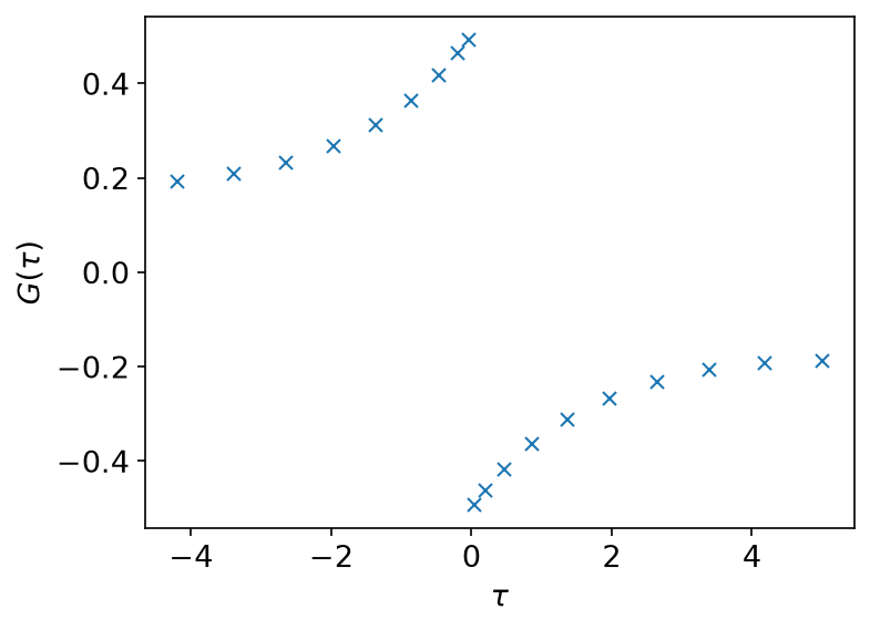
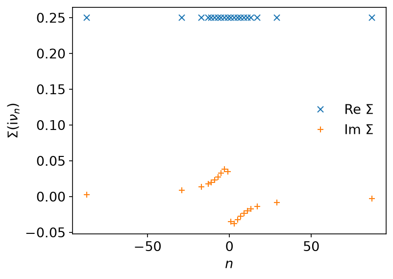
These signs are not the textbook ones. Since \(G(\tau) \le 0\) on \((0, \beta)\), \(P(\tau) = G(\tau) G(\beta - \tau)\) is positive; it is minus the usual single-spin bubble \(G(\tau) G(-\tau)\). The textbook self-energy is \(\Sigma = -GW\), with a spin sum in \(P\). The two sign changes cancel at order \(U^2\), so the second-order term has the textbook sign; the higher-order terms of the screening series do not. The example is about the structure of the loop — which product lives in which representation — not a quantitatively faithful \(GW\) for this model.
Only the constant part of \(W\) is split off: what is carried into
\(\Sigma\) is \(U/(1 - UP) - U\). The instantaneous part \(U\) would
give the static term \(U G(\beta^-) = -U\langle n \rangle\), with
\(\langle n\rangle\) the occupation per spin. In Hedin’s equations that is
the exchange (Fock) term, not the Hartree term; the code calls it hartree
after the notebook. It is computed separately and kept out of the Dyson
equation, because a constant only shifts the chemical potential.
Two statistics, one loop
\(G\) and \(\Sigma\) are fermionic; \(P\) and \(W\) are bosonic. The two products mix them: \(P\) is a product of \(G\)’s evaluated at the bosonic sampling times, and \(\Sigma\) needs \(W\) at the fermionic ones. So the example carries two bases and two meshes:
    // Two bases with the same Λ = βω_max. `new` runs the SVE for each; for a
    // larger Λ, compute it once and use `FiniteTempBasis::from_sve_result`.
    let basis_f = FiniteTempBasis::<LogisticKernel, Fermionic>::new(
        LogisticKernel::new(BETA * WMAX)?,
        BETA,
        None,
        None,
    )?;
    let basis_b = FiniteTempBasis::<LogisticKernel, Bosonic>::new(
        LogisticKernel::new(BETA * WMAX)?,
        BETA,
        None,
        None,
    )?;
    let mesh_f = IrMesh::<Fermionic>::new(&basis_f)?;
    let mesh_b = IrMesh::<Bosonic>::new(&basis_b)?;
Both bases use the same kernel, so they could share one singular value
expansion. Calling FiniteTempBasis::new twice computes it twice; at
\(\Lambda = 10\) that costs nothing, but for a large \(\Lambda\) compute the
SVE once and build both bases with FiniteTempBasis::from_sve_result, as
Conventions shows.
The loop also needs two evaluation matrices, built once outside it, and the row \(u_l(\beta^-)\) for the static term:
    // The two cross-statistics evaluation matrices, built once: the fermionic
    // basis functions at the bosonic sampling times, and the other way round.
    let uf_at_tau_b = basis_f.evaluate_tau(mesh_b.tau_points())?;
    let ub_at_tau_f = basis_b.evaluate_tau(mesh_f.tau_points())?;
    // u_l(β⁻), for the Hartree term.
    let uf_at_beta = basis_f.evaluate_tau(&[BETA])?;
Basis::evaluate_tau is the operation that makes this safe. The sampling
times live on \([-\beta/2, \beta/2]\), so evaluating a basis function there
needs the (anti-)periodicity relation — and which relation is a property of
the function, never of the grid it is being sampled on. \(G\) stays
anti-periodic when evaluated at bosonic times; \(W\) stays periodic at
fermionic ones. evaluate_tau applies the statistics of the basis it belongs
to, which is exactly right. Doing the same thing by hand — folding the times
and then multiplying by a sign taken from the grid — is the mistake this
example exists to rule out.
The reversal, again
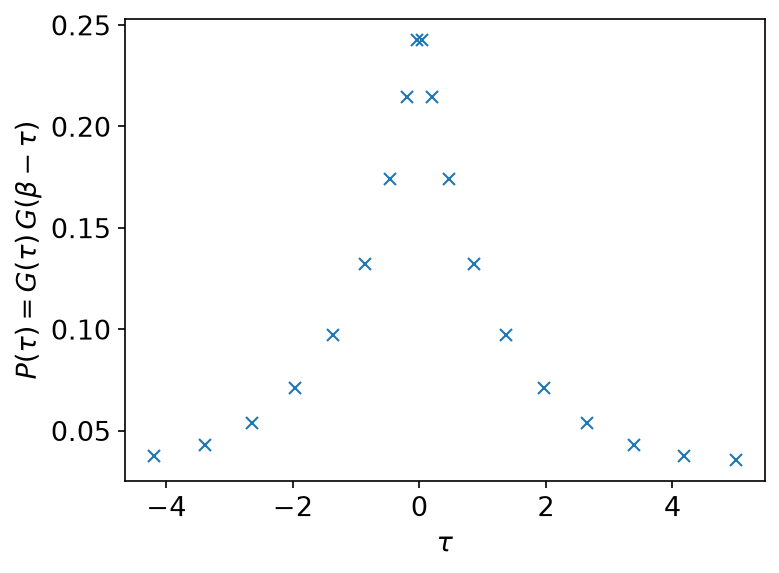
\(P(\tau) = G(\tau) G(\beta - \tau)\) needs the same reversal as the second-order self-energy, and here it has a wrinkle. At \(\beta = 10\), \(\omega_\mathrm{max} = 1\) and the default accuracy, both grids hold 19 points: 18 of them in \(\pm\) pairs, and one at exactly \(\tau = \beta/2\). That last point has no partner under \(\tau \to -\tau\) on the grid — its mirror \(-\beta/2\) is the same point one period away. The reversal must therefore allow for a wrap, which brings a second \(\zeta\); at \(\beta/2\) the two cancel and the row maps to itself with a plus sign.
evaluate_rows (a tutorial helper) contracts a matrix of basis-function
values with a block of coefficients:
        let g_tau_b = evaluate_rows(&uf_at_tau_b, &g_l_f, 1);
        // P(τ) = G(τ) G(β − τ), with G(β − τ) = −G(−τ): the reversed array
        // with the *fermionic* sign, even though the times are the bosonic
        // ones. This grid also carries a point at exactly τ = β/2, whose
        // mirror is itself one period away; `reverse_tau_as` handles that.
        let g_beta_minus_tau = mesh_b.reverse_tau_as::<Fermionic>(&g_tau_b, 1);
        let p_tau_b: Vec<Complex64> = g_tau_b
            .iter()
            .zip(&g_beta_minus_tau)
            .map(|(g, g_reversed)| g * g_reversed)
            .collect();
        let p_l_b = mesh_b.tau_to_l(&p_tau_b, 1)?;
        let p_iw_b = mesh_b.l_to_wn(&p_l_b, 1)?;
For this particular model the check is worth stating plainly: the model is particle-hole symmetric, so \(G(\beta - \tau) = G(\tau)\) and a plot of the two would show one curve. The fermionic and bosonic sampling times coincide as well, because the logistic kernel gives both statistics the same \(u_l(\tau)\). Neither the picture nor the abscissa would reveal a missing \(\zeta\) — only the numbers would.
The screened interaction
\(W\) is algebraic on the Matsubara axis and then has to come back to imaginary time — on the fermionic grid, because that is where it meets \(G\):
        // W = U/(1 − UP); only the frequency-dependent part U/(1 − UP) − U is
        // carried on, the constant being the bare interaction itself.
        let w_iw_b: Vec<Complex64> = p_iw_b.iter().map(|p| U / (1.0 - U * p) - U).collect();
        let w_l_b = mesh_b.wn_to_l(&w_iw_b, 1)?;
        // --- and back into fermionic statistics -------------------------------
        let w_tau_f = evaluate_rows(&ub_at_tau_f, &w_l_b, 1);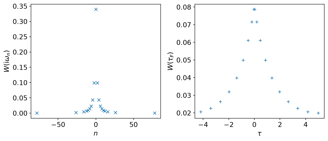
The self-energy, and the loop
        let e_tau_f: Vec<Complex64> = g_tau_f.iter().zip(&w_tau_f).map(|(g, w)| g * w).collect();
        let e_l_f = mesh_f.tau_to_l(&e_tau_f, 1)?;
        let e_iw_f = mesh_f.l_to_wn(&e_l_f, 1)?;
        // The static term U G(β⁻) = −U⟨n⟩. The name follows the notebook; in
        // Hedin's equations this instantaneous piece is the exchange (Fock)
        // term. It is subtracted, so the reported Σ carries +U⟨n⟩.
        let hartree: Complex64 = U * evaluate_rows(&uf_at_beta, &g_l_f, 1)[0];
        let e_iw_f_hartree: Vec<Complex64> = e_iw_f.iter().map(|e| e - hartree).collect();
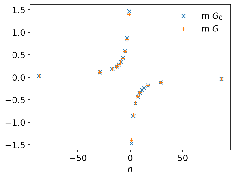
and the Dyson equation \(G = 1/(G_0^{-1} - \Sigma)\) closes the loop:
        // The Dyson equation. The static term is left out of it, as in the
        // notebook: it is a constant shift of the chemical potential.
        g_iw_f = g_iw_0
            .iter()
            .zip(&e_iw_f)
            .map(|(g0, e)| (g0.inv() - e).inv())
            .collect();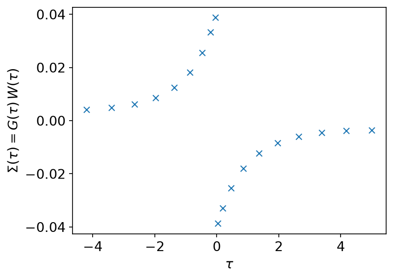
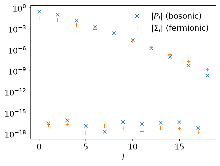
Both expansions fall off like the singular values of their own basis, which is the statement that a product of Green’s functions is still a function the basis represents well — the fact the whole method rests on:
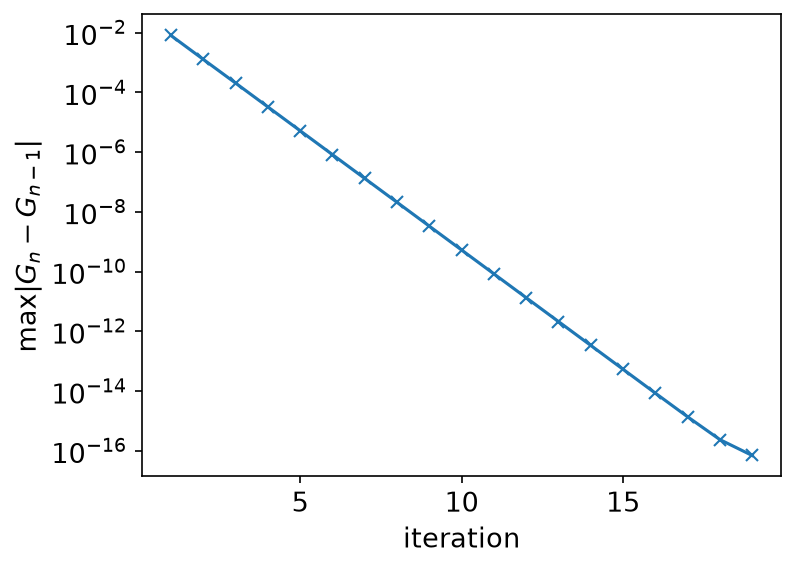
Twenty iterations are more than enough: the change in \(\Sigma\) falls by about a decade per step and reaches the rounding floor around iteration 18.
Going further
This page uses only the IR basis and stays on the imaginary axis. For real-frequency output, see MiniPole, which fits a few poles to Matsubara data by ESPRIT, and Analytic continuation for why that step is ill posed. The DLR page shows the pole-based representation of imaginary-axis data.
Running it
From docs/tutorial-code:
$ cargo run --release --bin gw
The program writes CSV tables to docs/tutorial-code/data/gw/. The figures
are drawn from those tables; from the repository root, run
uv run --project docs/plotting python docs/plotting/gw_plot.py. The reversal behind IrMesh::reverse_tau and reverse_tau_as
(reverse_tau_rows) is checked against a direct evaluation of
\(u_l(\beta - \tau)\) in docs/tutorial-code/tests/tau_convention.rs.
Key API pieces
From sparse-ir:
| What you want | What to call |
|---|---|
| a basis function of one statistics at the other’s sampling times | Basis::evaluate_tau |
| \(u_l(\beta^-)\), for the static term | Basis::evaluate_tau(&[beta]) |
| two bases from one SVE | compute_sve, then FiniteTempBasis::from_sve_result |
From the tutorial crate (sparse_ir_tutorial, not part of the library):
| What you want | What to call |
|---|---|
| \(G(\beta - \tau)\) for a function whose statistics is not the mesh’s | IrMesh::reverse_tau_as::<S> |
| the round trip through the basis | IrMesh::wn_to_l, l_to_tau, tau_to_l, l_to_wn |
| a matrix of basis-function values times a block of coefficients | evaluate_rows |
The whole loop is 19 + 19 coefficients wide. Nothing in it ever sees a dense imaginary-time grid.