Second-order perturbation
Ported from the Python notebook
second_order_perturbation_py.ipynb
of sparse-ir-tutorial.
The program that produced every number and figure on this page is
docs/tutorial-code/src/bin/second_order_perturbation.rs; the code below is
included from it.
This is the first page where the basis earns its keep on a real problem: the second-order self-energy of the Hubbard model on a square lattice, on a 256 × 256 momentum grid at \(\beta = 10^3\). Nothing here is ever stored on a dense imaginary-time or Matsubara grid — 70 basis functions carry the whole frequency dependence.
Theory
The Hubbard model at half filling,
\[ \mathcal{H} = -t \sum_{\langle i, j\rangle} c^\dagger_{i\sigma} c_{j\sigma}
- U \sum_i n_{i\uparrow} n_{i\downarrow}
- \mu \sum_i (n_{i\uparrow} + n_{i\downarrow}), \]
with \(t = 1\), \(U = 2\) and \(\mu = U/2\), has the non-interacting dispersion
\[ \epsilon(\boldsymbol{k}) = -2(\cos k_x + \cos k_y) \]
and the non-interacting Green’s function
\[ G(\mathrm{i}\nu_n, \boldsymbol{k}) = \frac{1}{\mathrm{i}\nu_n - \epsilon(\boldsymbol{k}) + \tilde\mu}, \qquad \nu_n = n\pi/\beta,\ n \text{ odd}. \]
Here \(\tilde\mu = \mu - U\langle n_{\bar\sigma}\rangle\) is the chemical potential shifted by the first-order (Hartree) self-energy. At half filling \(\langle n_{\bar\sigma}\rangle = 1/2\), so \(\mu = U/2\) gives \(\tilde\mu = 0\) and the dispersion is used as it stands. The second-order term is a product in imaginary time and real space:
\[ \Sigma(\tau, \boldsymbol{r}) = U^2 G^2(\tau, \boldsymbol{r}), G(\beta - \tau, \boldsymbol{r}). \]
That single line is the reason the calculation moves between representations. \(G\) is a formula on the Matsubara axis; the self-energy is a product only in \((\tau, \boldsymbol{r})\); and the answer is wanted back on the Matsubara axis. Each hop is one fit and one evaluation.
Momentum and real space are connected by
\[ A(\mathrm{i}\nu, \boldsymbol{r}) = \frac{1}{N} \sum_{\boldsymbol{k}} e^{-\mathrm{i}\boldsymbol{k}\cdot\boldsymbol{r}} A(\mathrm{i}\nu, \boldsymbol{k}), \qquad A(\mathrm{i}\nu, \boldsymbol{k}) = \sum_{\boldsymbol{r}} e^{\mathrm{i}\boldsymbol{k}\cdot\boldsymbol{r}} A(\mathrm{i}\nu, \boldsymbol{r}), \]
with \(N = N_\mathrm{lin}^2\) points on each of the two regular grids. Both are FFTs, which is what makes 65536 momenta affordable.
The basis and the sampling points
\(\Lambda = 10^5\), \(\beta = 10^3\) (so \(\omega_\mathrm{max} = 100\)) and \(\varepsilon = 10^{-7}\) give a basis of 70 functions, with 70 sampling times and 70 sampling frequencies.
use sparse_ir::{Fermionic, FermionicFreq, FiniteTempBasis, LogisticKernel, MatsubaraSampling};
const LAMBDA: f64 = 1e5;
const BETA: f64 = 1e3;
const EPS: f64 = 1e-7;
const WMAX: f64 = LAMBDA / BETA;
    let kernel = LogisticKernel::new(BETA * WMAX)?;
    let basis = FiniteTempBasis::<LogisticKernel, Fermionic>::new(kernel, BETA, Some(EPS), None)?;
Ok::<(), Box<dyn std::error::Error>>(())
The condition numbers of the two samplings are about 163 and 466, so a fit loses two to three significant digits: with \(\varepsilon = 10^{-7}\) the results are good to four or five. Asking for a smaller \(\varepsilon\) buys more of them, at the price of a larger basis.
The example wraps the two samplings in an IrMesh, a small helper of the
tutorial crate that holds a TauSampling and a MatsubaraSampling for one
basis and moves a whole array of Green’s functions between them:
    let mesh = IrMesh::<Fermionic>::new(&basis)?;
    let grid = MomentumGrid::new(NK_LIN, NK_LIN);
    let nk = grid.len();
Arrays are stored row-major as (frequency or time, momentum), so nk is the
column count every transform is told about.
From the Matsubara axis to \((\tau, \boldsymbol{r})\)
\(G_0\) is written down frequency by frequency, at the sampling frequencies of the mesh,
    let ek = grid.square_lattice_dispersion(1.0);
    // ν_n = nπ/β, with the reduced (odd) index n of the sampling frequencies.
    let nu: Vec<f64> = mesh.wn().iter().map(|w| w.n() as f64 * PI / BETA).collect();
    // G₀(iν, k) = 1/(iν − ε(k)), stored row-major as (frequency, momentum).
    let mut gkf = Vec::with_capacity(mesh.n_wn() * nk);
    for &nu in &nu {
        for &e in &ek {
            gkf.push(Complex64::new(-e, nu).inv());
        }
    }
and then fitted to the basis, evaluated at the sampling times, and moved into real space:
    let gkl = mesh.wn_to_l(&gkf, nk)?; // values → coefficients
    assert_eq!(gkl.len(), basis.size() * nk);
    let gkt = mesh.l_to_tau(&gkl, nk)?; // coefficients → values
    let grt = grid.k_to_r(&gkt);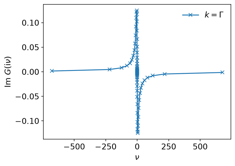
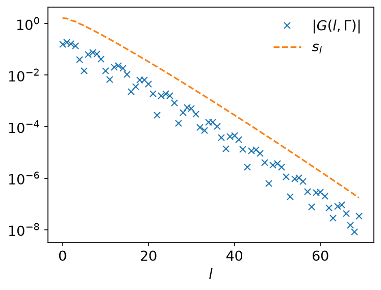
The coefficients fall off like the singular values, which is the statement that the basis is the right one for this function:
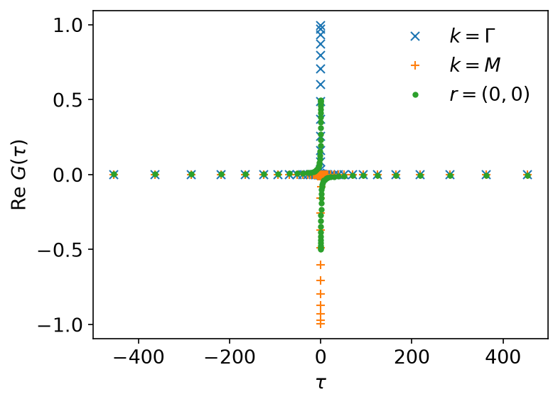
Note where the sampling times lie: on \([-\beta/2, \beta/2]\), not on \([0, \beta)\) as in the Python notebook. The two are the same set of points seen through \(G(\tau - \beta) = -G(\tau)\); see Conventions.
The self-energy
\(G(\beta - \tau)\) is where that convention has to be handled rather than
just noted. On \([0, \beta)\) it is the reversed array, which is what the
notebook writes as grt[::-1]. On the symmetric grid the reversed array is
\(G(-\tau)\), and
\[ G(\beta - \tau) = \zeta, G(-\tau), \qquad \zeta = -1 \text{ (fermionic)},\ +1 \text{ (bosonic)}, \]
so the sign has to come along. IrMesh::reverse_tau is exactly that
operation, and it is the only place in the applied tutorials where the
relation appears. It does not assume the grid is closed under
\(\tau \to -\tau\): a sampling time may sit at exactly \(\beta/2\), whose
mirror is the same point one period away, and the extra \(\zeta\) from that
period is applied where it is needed (see GW, whose grid has such a
point):
    // G(β − τ) on the symmetric grid: the reversed rows, times ζ = −1.
    let reversed = mesh.reverse_tau(&grt, nk);
    let srt: Vec<Complex64> = grt
        .iter()
        .zip(&reversed)
        .map(|(g, g_reversed)| U * U * g * g * g_reversed)
        .collect();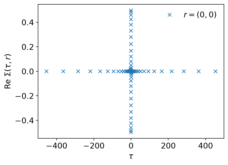
Getting the sign wrong, or reversing without it, changes \(\Sigma\) by a factor of order one — a picture that still looks plausible. So check the relation against a direct evaluation of \(u_l(\beta - \tau)\) rather than trusting a reading of the convention.
Back to the Matsubara axis
The way back is the way in, in reverse:
    let srl = mesh.tau_to_l(&srt, nk)?; // values → coefficients
    let skl = grid.r_to_k(&srl); // and back to momentum
    let sigma_iv = mesh.l_to_wn(&skl, nk)?;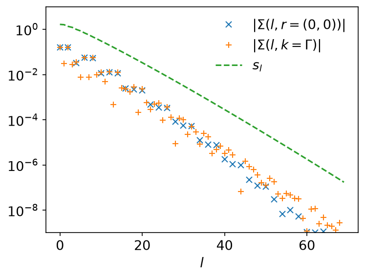
The coefficients of \(\Sigma\) decay like those of \(G\), which says the product of three Green’s functions is still a function the basis represents well — the fact the whole method rests on.
Because the answer is a set of coefficients, \(\Sigma\) can be evaluated on any frequencies at all, not only on the ones that were sampled. Here on every twentieth fermionic frequency out to \(|n| \approx 20000\): the textbook index \(m\) runs in steps of 20, so the reduced index \(n = 2m + 1\) runs in steps of 40, from \(-19999\) to \(19961\).
    // The coefficients are the whole answer: Σ can be evaluated on any
    // frequency, not only on the ones that were sampled. Here, every twentieth
    // fermionic frequency (m in steps of 20, so n = 2m + 1 in steps of 40) out
    // to |n| ≈ 20000 — far beyond the sampling set.
    let far: Vec<i64> = (-10000..10000).step_by(20).map(|n| 2 * n + 1).collect();
    let freqs: Vec<FermionicFreq> = far
        .iter()
        .map(|&n| FermionicFreq::new(n))
        .collect::<Result<_, _>>()?;
    let sampling = MatsubaraSampling::<Fermionic>::with_sampling_points(&basis, freqs)?;
    // Only Γ is wanted, so evaluate one column rather than all of them.
    let skl_gamma: Vec<Complex64> = (0..basis.size()).map(|l| skl[l * nk + gamma]).collect();
    let sigma_far = sampling.evaluate(&skl_gamma)?;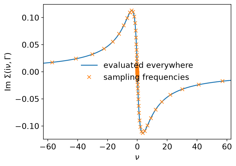
The sampled points lie on the evaluated curve, which is the whole claim: 70 numbers per momentum hold the frequency dependence of \(\Sigma\) everywhere.
Going further
This page uses only the IR basis and stays on the imaginary axis. For real-frequency output, see MiniPole, which fits a few poles to Matsubara data by ESPRIT, and Analytic continuation for why that step is ill posed. The DLR page shows the pole-based representation of imaginary-axis data.
Running it
From docs/tutorial-code:
$ cargo run --release --bin second_order_perturbation
The program writes CSV tables to docs/tutorial-code/data/second_order_perturbation/.
The figures are drawn from those tables; from the repository root, run
uv run --project docs/plotting python docs/plotting/second_order_perturbation_plot.py.
The reversal behind IrMesh::reverse_tau and reverse_tau_as
(reverse_tau_rows) is checked against a direct evaluation of
\(u_l(\beta - \tau)\) in docs/tutorial-code/tests/tau_convention.rs.
Key API pieces
From sparse-ir:
| What you want | What to call |
|---|---|
| values at the sampling frequencies → coefficients | MatsubaraSampling::fit_nd |
| coefficients → values at the sampling times | TauSampling::evaluate_nd_zz |
| the same, for a whole array of momenta | the _nd variants, with the momentum axis as the columns |
| \(\Sigma\) on frequencies you choose | MatsubaraSampling::with_sampling_points |
From the tutorial crate (sparse_ir_tutorial, not part of the library):
| What you want | What to call |
|---|---|
| both samplings of one basis, applied to a block of columns | IrMesh::wn_to_l, l_to_tau, tau_to_l, l_to_wn |
| \(G(\beta - \tau)\) on the symmetric grid | IrMesh::reverse_tau (reverse the rows, apply \(\zeta\)) |
| FFTs between momentum and real space | MomentumGrid::k_to_r, r_to_k |
The _nd variants are what keep this example fast: one call moves all 65536
momenta between representations, where a loop over evaluate would pay the
setup cost 65536 times.