TPSC approximation#
Author: Niklas Witt
Theory of TPSC#
The Two-Particle Self-Consistent (TPSC) approximation is a non-perturbative semi-analytical method that was first introduced by Vilk and Tremblay [Vilk and Tremblay, 1997]. TPSC can be used to study magnetic fluctuations, while it also obeys the Mermin-Wagner theorem in two dimensions, i.e., a phase transtition at finite temperatures is prohibited. In addition, the TPSC method satisfies several conservation laws, sum rules and the Pauli principle (actually, it is constructed in a way to fulfill these, since they are used to determine model parameters self-consistently). TPSC is applicable in the weak to intermediate coupling regime, but it breaks down in the strong coupling regime and it cannot describe the Mott transition unlike other non-perturbative methods like Dynamical Mean-Field Theory (DMFT).
For a (pedagogical) review, please have a look at [Allen et al., 2004] for the single-orbital case implemented here and [Zantout et al., 2021] for the more complex multi-orbital theory.
Set of TPSC equations#
We review the set of equations that need to be solved in the TPSC approximation assuming a one-band Hubbard model with interaction \(U\) (it is not so easy to extend TPSC to models with more parameters, since sum rules to determine the additional parameters self-consistently need to be found) in the paramagnetic phase (SU(2) symmetric), i.e., \(n = \langle n\rangle = 2n_{\sigma}\) for the electron filling \(n\). TPSC is constructed in a way to fulfill certain sum rules and the Pauli principle in the form \(\langle n^2\rangle = \langle n\rangle\). The control quantitites are spin and charge correlation function (susceptibilities) which are evaluated in a Random-Phase-Approximation (RPA) like fashion
with the irreducible susceptibility (“bubble diagram”)
where \(i\nu_m = 2n\pi T\) [\(i\omega_n=(2n+1)\pi T\)] and \(\boldsymbol{q}\) [\(\boldsymbol{k}\)] are bosonic [fermionic] Matsubara frequencies and momentum at temperature \(T\), \(N_{\boldsymbol{k}}\) denotes the number of \(\boldsymbol{k}\)-points, and \(G_0(i\omega_n,\boldsymbol{k}) = [i\omega_n - (\varepsilon_{\boldsymbol{k}}-\mu)]^{-1}\) is the bare (non-interacting) Green function with with single-particle dispersion \(\varepsilon_{\boldsymbol{k}}\) and chemical potential \(\mu\). Please note that sometimes a factor of 2 is included in the definition of \(\chi_0\) leading to slightly different factors in all equations given here. The convolution sum to calculate \(\chi_0\) can be easily evaluated by Fourier transforming to imaginary time and real space, resulting in a simple multiplication
In our practical implementation, we will perform this step using the sparse-ir package. A similar calculation is necessary to set the chemical potential \(\mu\) for fixed electron density \(n\), as
with a factor 2 from spin degeneracy and \(0^+ = \lim_{\eta\to 0+} \eta\) needs to be solved by using some root finding algorithm like bisection method or Brent’s method. The Fourier transformation to \(\tau=0^+\) can be easily performed with the sparse-ir package.
The above RPA definition of spin and charge susceptibility violate the Pauli principle. In TPSC, we overcome this problem by introducing two effective, renormalized interactions (“irreducible vertices”) \(U_{\mathrm{sp}}\) and \(U_{\mathrm{ch}}\) that enter spin and charge correlation functions as
These two effetive interactions are determined by the two local sum rules
Both sum rules can be exactly derived from the Pauli principle (\(\langle n^2\rangle = \langle n\rangle\)). In principle, we could now determine \(U_{\mathrm{sp}}\) and \(U_{\mathrm{ch}}\) from local-spin and local-charge sum rule if we knew the double occupancy \(\langle n_{\uparrow}n_{\downarrow}\rangle\). TPSC makes the ansatz
which reproduces Kanamori-Brueckner type screening. The four equations above form a set of self-consistent equations for either \(U_{\mathrm{sp}}\) or equivalently \(\langle n_{\uparrow}n_{\downarrow}\rangle\). In practice, we treat \(U_{\mathrm{sp}}\) as the parameter to be determined self-consistently by inserting the ansatz in the local-spin sum rule. Effectively, we then need to find the root of the function
Afterwards we can calculate the double occupancy \(\langle n_{\uparrow}n_{\downarrow}\rangle = \frac{U_{\mathrm{sp}}}{4U} n^2\) and then perform a similar root finding for \(U_{\mathrm{ch}}\) from the function
In TPSC, a self-energy \(\Sigma\) can be derived that is calculated from the interaction [Moukouri et al., 2000]
The self-energy itself is given by a convolution in \((i\omega_n, \boldsymbol{k})\) space
which Fourier transformed to \((\tau,\boldsymbol{r})\) space takes the form
The interacting Green function is determined by the Dyson equation
Practical implementation#
When implementing the TPSC, a few points need to be treated carefully which we discuss in the following.
The constant Hartree term \(V_{\mathrm{H}} = U\) in the interaction \(V\) and respective self-energy term \(\Sigma_H = U n_{\sigma} = U\frac{n}{2}\) can be absorbed into the definition of the chemical potential \(\mu\).
An upper bound for the renormalized spin vertex \(U_{\mathrm{sp}}\) exists. Since the denominator spin susceptibility \(\chi_{\mathrm{sp}}\) should not diverge, the upper bound is given by the RPA critical interaction value \(U_{\mathrm{crit}} = 1/\mathrm{max}\{\chi^0\}\). Mathematically, the function \(f(U_{\mathrm{sp}}) = 2\sum \chi_{\mathrm{sp}}(U_{\mathrm{sp}}) - n + \frac{U_{\mathrm{sp}}}{2U}n^2\), from which \(U_{\mathrm{sp}}\) is determined, turns unstable for \(U_{\mathrm{sp}} \geq U_{\mathrm{crit}}\) (try plotting \(f(U_{\mathrm{sp}})\)!). At this point, TPSC is not applicable and, e.g., the temperature \(T\) is too low or the (unrenormalized) interaction \(U\) too large.
An internal accuracy check \(\frac{1}{2}\mathrm{Tr}(\Sigma G) = U \langle n_{\uparrow} n_{\downarrow}\rangle\) can be employed to test the validity of TPSC.
Code implementation#
We are implementing TPSC for the simple case of a square lattice model with dispersion \(\varepsilon_{\boldsymbol{k}} = -2t\,[\cos(k_x) + \cos(k_y)]\) with nearest-neighbor hopping \(t\) which sets the energy scale of our system (bandwidth \(W = 8t\)). First, we load all necessary basic modules that we are going to need in implementing TPSC and visualizing results:
import numpy as np
import scipy as sc
import scipy.optimize
from warnings import warn
import sparse_ir
%matplotlib inline
import matplotlib.pyplot as plt
Parameter setting#
### System parameters
t    = 1      # hopping amplitude
W    = 8*t    # bandwidth
wmax = 10     # set wmax >= W

T    = 0.1    # temperature
beta = 1/T    # inverse temperature
n    = 0.85   # electron filling, here per spin per lattice site (n=1: half filling)
U    = 4      # Hubbard interaction

### Numerical parameters
nk1, nk2  = 24, 24    # number of k_points along one repiprocal crystal lattice direction k1 = kx, k2 = ky
nk        = nk1*nk2
IR_tol    = 1e-10     # accuary for l-cutoff of IR basis functions
Generating meshes#
We need to generate a \(\boldsymbol{k}\)-mesh as well as set up the IR basis functions on a sparse \(\tau\) and \(i\omega_n\) grid. Then we can calculate the dispersion on this mesh. In addition, we set calculation routines to Fourier transform \(k\leftrightarrow r\) and \(\tau\leftrightarrow i\omega_n\) (via IR basis).
#### Initiate fermionic and bosonic IR basis objects
IR_basis_set = sparse_ir.FiniteTempBasisSet(beta, wmax, eps=IR_tol)

class Mesh:
    """
    Holding class for k-mesh and sparsely sampled imaginary time 'tau' / Matsubara frequency 'iw_n' grids.
    Additionally it defines the Fourier transform routines 'r <-> k'  and 'tau <-> l <-> wn'.
    """
    def __init__(self,IR_basis_set,nk1,nk2):
        self.IR_basis_set = IR_basis_set

        # generate k-mesh and dispersion
        self.nk1, self.nk2, self.nk = nk1, nk2, nk1*nk2
        self.k1, self.k2 = np.meshgrid(np.arange(self.nk1)/self.nk1, np.arange(self.nk2)/self.nk2)
        self.ek = -2*t*( np.cos(2*np.pi*self.k1) + np.cos(2*np.pi*self.k2) ).reshape(nk)

        # lowest Matsubara frequency index
        self.iw0_f = np.where(self.IR_basis_set.wn_f == 1)[0][0]
        self.iw0_b = np.where(self.IR_basis_set.wn_b == 0)[0][0]

        ### Generate a frequency-momentum grid for iw_n and ek (in preparation for calculating the Green function)
        # frequency mesh (for Green function)
        self.iwn_f = 1j * self.IR_basis_set.wn_f * np.pi * T
        self.iwn_f_ = np.tensordot(self.iwn_f, np.ones(nk), axes=0)

        # ek mesh
        self.ek_ = np.tensordot(np.ones(len(self.iwn_f)), self.ek, axes=0)

    def smpl_obj(self, statistics):
        """ Return sampling object for given statistic """
        smpl_tau = {'F': self.IR_basis_set.smpl_tau_f, 'B': self.IR_basis_set.smpl_tau_b}[statistics]
        smpl_wn  = {'F': self.IR_basis_set.smpl_wn_f,  'B': self.IR_basis_set.smpl_wn_b }[statistics]
        return smpl_tau, smpl_wn


    def tau_to_wn(self, statistics, obj_tau):
        """ Fourier transform from tau to iw_n via IR basis """
        smpl_tau, smpl_wn = self.smpl_obj(statistics)

        obj_tau = obj_tau.reshape((smpl_tau.tau.size, self.nk1, self.nk2))
        obj_l   = smpl_tau.fit(obj_tau, axis=0)
        obj_wn  = smpl_wn.evaluate(obj_l, axis=0).reshape((smpl_wn.wn.size, self.nk))
        return obj_wn

    def wn_to_tau(self, statistics, obj_wn):
        """ Fourier transform from tau to iw_n via IR basis """
        smpl_tau, smpl_wn = self.smpl_obj(statistics)

        obj_wn  = obj_wn.reshape((smpl_wn.wn.size, self.nk1, self.nk2))
        obj_l   = smpl_wn.fit(obj_wn, axis=0)
        obj_tau = smpl_tau.evaluate(obj_l, axis=0).reshape((smpl_tau.tau.size, self.nk))
        return obj_tau


    def k_to_r(self,obj_k):
        """ Fourier transform from k-space to real space """
        obj_k = obj_k.reshape(-1, self.nk1, self.nk2)
        obj_r = np.fft.fftn(obj_k,axes=(1,2))
        obj_r = obj_r.reshape(-1, self.nk)
        return obj_r

    def r_to_k(self,obj_r):
        """ Fourier transform from real space to k-space """
        obj_r = obj_r.reshape(-1, self.nk1, self.nk2)
        obj_k = np.fft.ifftn(obj_r,axes=(1,2))/self.nk
        obj_k = obj_k.reshape(-1, self.nk)
        return obj_k
/opt/hostedtoolcache/Python/3.8.18/x64/lib/python3.8/site-packages/sparse_ir/basis.py:232: UserWarning:
Requested accuracy is 1e-10, which is below the
accuracy 1e-08 for the work data type <class 'numpy.float64'>.
Expect singular values and basis functions for large l to
have lower precision than the cutoff.
Install the xprec package to gain more precision.

  sve_result = sve.compute(_kernel.LogisticKernel(beta*wmax), eps)
TPSC solver#
We wrap the calculation steps of TPSC (i.e. determining \(U_{\mathrm{sp}},U_{\mathrm{ch}}\)) in a Solver class. We use the Mesh class defined above to perform calculation steps.
class TPSCSolver:
    def __init__(self, mesh, U, n, U_sfc_tol=1e-12, verbose=True):
        """
        Solver class to calculate the TPSC method.
        After initializing the Solver by `solver = TPSCSolver(mesh, U, n, **kwargs)` it
        can be run by `solver.solve()`.
        """
        ## set internal parameters for the solve
        self.U = U
        self.n = n
        self.mesh = mesh
        self.U_sfc_tol = U_sfc_tol
        self.verbose = verbose

        ## set initial Green function and irreducible susceptibility
        # NOT running the TPSCSolver.solve instance corresponds to staying on RPA level
        self.sigma = 0

        self.mu = 0
        self.mu_calc()

        self.gkio_calc(self.mu)
        self.grit_calc()
        self.ckio_calc()

        # determine critical U_crit = 1/max(chi0) as an upper bound to U_sp
        self.U_crit = 1/np.amax(self.ckio.real)


    #%%%%%%%%%%% Solving instance
    def solve(self):
        """
        Determine spin and charge vertex self-consistently from sum rules and calculate self-energy.
        """
        # determine spin vertex U_sp
        self.spin_vertex_calc()

        # set double occupancy from Kanamori-Bruckner screening
        self.docc_calc()

        # determine charge vertex U_ch
        self.charge_vertex_calc()

        # set spin and charge susceptibility
        self.chi_spin   = self.RPA_term_calc( self.U_sp)
        self.chi_charge = self.RPA_term_calc(-self.U_ch)

        # calculate interaction, self-energy and interacting Green function
        self.V_calc()
        self.sigma_calc()
        self.mu_calc()
        self.gkio_calc(self.mu)

    #%%%%%%%%%%% Calculation steps for self.energy
    def gkio_calc(self, mu):
        """ Calculate Green function G(iw,k) """
        self.gkio = (self.mesh.iwn_f_ - (self.mesh.ek_ - mu) - self.sigma)**(-1)

    def grit_calc(self):
        """ Calculate real space Green function G(tau,r) [for calculating chi0 and sigma] """
        # Fourier transform
        grit = self.mesh.k_to_r(self.gkio)
        self.grit = self.mesh.wn_to_tau('F', grit)

    def ckio_calc(self):
        """ Calculate irreducible susciptibility chi0(iv,q) """
        ckio = self.grit * self.grit[::-1, :]

        # Fourier transform
        ckio = self.mesh.r_to_k(ckio)
        self.ckio = self.mesh.tau_to_wn('B', ckio)

    def V_calc(self):
        """ Calculate interaction V(tau,r) from RPA-like spin and charge susceptibility """
        V = self.U/4 * (3*self.U_sp*self.chi_spin + self.U_ch*self.chi_charge)
        # Constant Hartree Term V ~ U needs to be treated extra, since they cannot be modeled by the IR basis.
        # In the single-band case, the Hartree term can be absorbed into the chemical potential.

        # Fourier transform
        V = self.mesh.k_to_r(V)
        self.V = self.mesh.wn_to_tau('B', V)

    def sigma_calc(self):
        """ Calculate self-energy Sigma(iwn,k) """
        sigma = self.V * self.grit

        # Fourier transform
        sigma = self.mesh.r_to_k(sigma)
        self.sigma = self.mesh.tau_to_wn('F', sigma)


    #%%%%%%%%%%% Determining spin and charge vertex
    def RPA_term_calc(self, U):
        """ Set RPA-like susceptibility """
        chi_RPA = self.ckio / (1 - U*self.ckio)
        return chi_RPA

    def chi_qtrace_calc(self, U):
        """ Calculate (iv_m, q) trace of chi_RPA term """
        # chi_qtrace = sum_(m,q) chi(iv_m,q)
        chi_RPA = self.RPA_term_calc(U)
        chi_trace = np.sum(chi_RPA, axis=1)/self.mesh.nk
        chi_trace_l  = self.mesh.IR_basis_set.smpl_wn_b.fit(chi_trace)
        chi_trace = self.mesh.IR_basis_set.basis_b.u(0)@chi_trace_l
        return chi_trace.real

    def docc_calc(self):
        """ Calculate double occupancy from Kanamori-Bruckner type screening """
        self.docc = 0.25 * self.U_sp/self.U * self.n**2

    def spin_vertex_calc(self):
        """ Determine self-consistently from sum rule """
        # interval [U_a, U_b] for root finding
        U_a = 0
        U_b = np.floor(self.U_crit*100)/100

        chi_trace = self.chi_qtrace_calc
        sfc_eq = lambda U_sp : 2*chi_trace(U_sp) - self.n + 0.5*(U_sp/self.U)*self.n**2

        if sfc_eq(U_b) > 0:
            self.U_sp = sc.optimize.brentq(sfc_eq, U_a, U_b, rtol = self.U_sfc_tol)
        else:
            warn("System underwent phase transition, U^sp > U_crit = {}! U is too large or T too low for given doping.".format(self.U_crit))

    def charge_vertex_calc(self):
        """ Determine self-consistently from sum rule """
        # interval [U_a, U_b] for root finding
        U_a = 0
        U_b = 100

        chi_trace = self.chi_qtrace_calc
        sfc_eq = lambda U_ch : 2*chi_trace(-U_ch) - self.n + (1 - 2*self.docc)*self.n**2

        self.U_ch = sc.optimize.brentq(sfc_eq, U_a, U_b, rtol = self.U_sfc_tol)


    #%%%%%%%%%%% Setting chemical potential mu
    def calc_electron_density(self, mu):
        """ Calculate chemical potential mu from Green function """
        self.gkio_calc(mu)
        gio  = np.sum(self.gkio,axis=1)/self.mesh.nk
        g_l  = self.mesh.IR_basis_set.smpl_wn_f.fit(gio)
        g_tau0 = self.mesh.IR_basis_set.basis_f.u(0)@g_l

        n  = 1 + np.real(g_tau0)
        n  = 2*n #for spin
        return n

    def mu_calc(self):
        """ Find chemical potential for a given filling n0 via brentq root finding algorithm """
        n_calc = self.calc_electron_density
        n0 = self.n
        f  = lambda mu : n_calc(mu) - n0

        self.mu = sc.optimize.brentq(f, np.amax(self.mesh.ek)*3, np.amin(self.mesh.ek)*3)
Execute TPSC solver#
# initialize calculation
IR_basis_set = sparse_ir.FiniteTempBasisSet(beta, wmax, eps=IR_tol)
mesh = Mesh(IR_basis_set, nk1, nk2)
solver = TPSCSolver(mesh, U, n)

# perform TPSC calculations
solver.solve()
Visualize results#
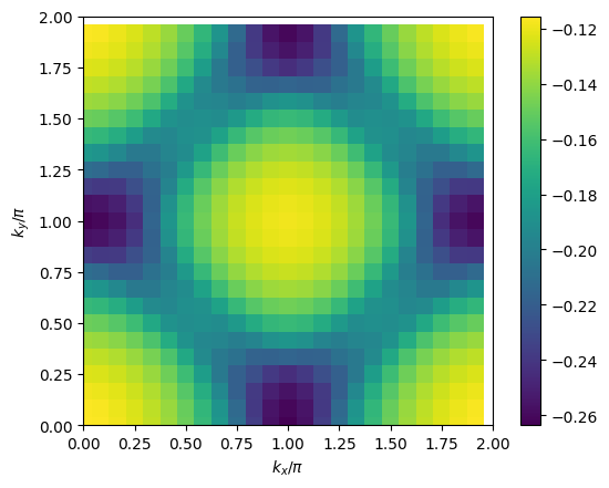
# plot 2D k-dependence of lowest Matsubara frequency of e.g. green function
plt.pcolormesh(2*mesh.k1.reshape(nk1,nk2), 2*mesh.k2.reshape(nk1,nk2), np.real(solver.gkio[mesh.iw0_f].reshape(mesh.nk1,mesh.nk2)), shading='auto')
ax = plt.gca()
ax.set_xlabel('$k_x/\pi$')
ax.set_xlim([0,2])
ax.set_ylabel('$k_y/\pi$')
ax.set_ylim([0,2])
ax.set_aspect('equal')
plt.colorbar()
plt.show()
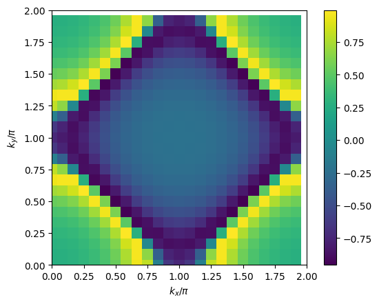
# plot 2D k-dependence of lowest Matsubara frequency of e.g. self-energy
plt.pcolormesh(2*mesh.k1.reshape(nk1,nk2), 2*mesh.k2.reshape(nk1,nk2), np.imag(solver.sigma[mesh.iw0_f].reshape(mesh.nk1,mesh.nk2)), shading='auto')
ax = plt.gca()
ax.set_xlabel('$k_x/\pi$')
ax.set_xlim([0,2])
ax.set_ylabel('$k_y/\pi$')
ax.set_ylim([0,2])
ax.set_aspect('equal')
plt.colorbar()
plt.show()
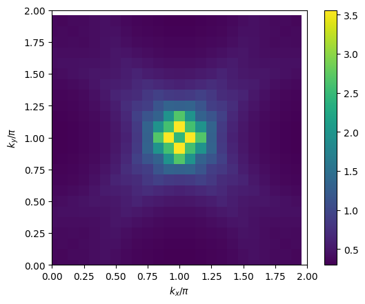
# plot 2D k-dependence of lowest Matsubara frequency of e.g. chi_spin
plt.pcolormesh(2*mesh.k1.reshape(nk1,nk2), 2*mesh.k2.reshape(nk1,nk2), np.real(solver.chi_spin[mesh.iw0_b].reshape(mesh.nk1,mesh.nk2)), shading='auto')
ax = plt.gca()
ax.set_xlabel('$k_x/\pi$')
ax.set_xlim([0,2])
ax.set_ylabel('$k_y/\pi$')
ax.set_ylim([0,2])
ax.set_aspect('equal')
plt.colorbar()
plt.show()
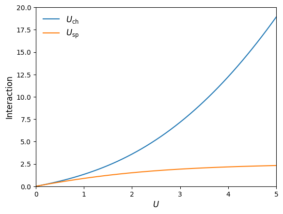
Example: Interaction dependent renormalization#
As a simple example demonstration of our SparseIR TPSC code developed above, we will reproduce Fig. 2 of []. It shows the \(U\) dependence of renormalized/effective spin and charge interactions \(U_{\mathrm{sp}}\) and \(U_{\mathrm{ch}}\) (irreducible vertices) at half filling \(n=1\) and \(T>T_{\mathrm{crit}}\) for all considered \(U\) (i.e. \(U_{\mathrm{sp}}<U_{\mathrm{crit}}\) is ensured).
You can simply execute the following two code blocks which will first perform the calculatn and then generate a figure like in the reference above.
#%%%%%%%%%%%%%%% Parameter settings
print('Initialization...')
# system parameters
t = 1         # hopping amplitude
n = 1         # electron filling, here per spin per lattice site (n=1: half filling)
T = 0.4       # temperature
beta =1/T
U_array = np.linspace(1e-10,5,51)  # Hubbard interaction

W    = 8*t    # bandwidth
wmax = 10     # set wmax >= W

# numerical parameters
nk1, nk2  = 24, 24    # k-mesh sufficiently dense!
nk        = nk1*nk2
IR_tol    = 1e-8      # accuary for l-cutoff of IR basis functions


# initialize meshes
IR_basis_set = sparse_ir.FiniteTempBasisSet(beta, wmax, eps=IR_tol)
mesh = Mesh(IR_basis_set, nk1, nk2)

# set initial self_energy - will be set to previous calculation step afterwards
sigma_init = 0

# empty arrays for results later
U_sp_array = np.empty((len(U_array)))
U_ch_array = np.empty((len(U_array)))


#%%%%%%%%%%%%%%% Calculations for different U values
print("Start TPSC loop...")
for U_it, U in enumerate(U_array):
    #print("Now: U = {:.1f}".format(U))

    # TPSC solver
    solver = TPSCSolver(mesh, U, n, verbose=False)
    solver.solve()

    # save data for plotting
    U_sp_array[U_it] = solver.U_sp
    U_ch_array[U_it] = solver.U_ch
print("Finished. Plotting now.")


#%%%%%%%%%%%%%%%% Plot results
plt.plot(U_array, U_ch_array, '-', label='$U_{\mathrm{ch}}$')
plt.plot(U_array, U_sp_array, '-', label='$U_{\mathrm{sp}}$')
ax = plt.gca()
ax.set_xlabel('$U$', fontsize=12)
ax.set_xlim([0,5])
ax.set_ylabel('Interaction', fontsize=12)
ax.set_ylim([0,20])
ax.legend(frameon=False, fontsize=12)
Initialization...
Start TPSC loop...
Finished. Plotting now.
<matplotlib.legend.Legend at 0x7f8493ea65e0>