The GF2 & GW method#
import numpy as np
import matplotlib.pyplot as pl
import sparse_ir
import sys
import math
T = 0.1
wmax = 1

beta = 1/T
#construction of the Kernel K

# Fermionic Basis

basisf = sparse_ir.FiniteTempBasis('F', beta, wmax)

matsf = sparse_ir.MatsubaraSampling(basisf)
tausf = sparse_ir.TauSampling(basisf)

# Bosonic Basis

basisb = sparse_ir.FiniteTempBasis('B', beta, wmax)

matsb = sparse_ir.MatsubaraSampling(basisb)
tausb = sparse_ir.TauSampling(basisb)

# Note:
# * The distribution of sampling times is symmetric around beta/2.
# * By default, the same sampling times are used for the fermioc and bosonic cases.
/opt/hostedtoolcache/Python/3.8.18/x64/lib/python3.8/site-packages/sparse_ir/basis.py:51: UserWarning: xprec package is not available:
expect single precision (1.5e-8) only as both cutoff and
accuracy of the basis functions
  warn("xprec package is not available:\n"
def rho(x):
    return 2/np.pi*np.sqrt(1-(x/wmax)**2)

rho_l = basisf.v.overlap(rho)

G_l_0 = -basisf.s*rho_l


# We compute G_iw two times as we will need G_iw_0 as a constant later on
G_iw_0 = matsf.evaluate(G_l_0)
G_iw_f = matsf.evaluate(G_l_0)
# Iterations
i = 0

# storage for E_iw to show convergence after iterations
E_iw_f_arr = []
Above we have successfully derived \(G^F(\bar{\tau}_k^F)\) from \(\hat {G}^F(i\bar{\omega}_n^F)\) by first obtaining the Green’s function’s basis representation \(G_l^F\) and secondly evaluating \(G_l^F\) on the \(\tau\)-sampling points, which are given by the computations of sparse_ir. Here, the self-consistent second order Green’s function theory (GF2) and the self-consistent GW methodare are based this very mechanism (and the so called Hedin equations).[5][7]
The following image should give an overview on their iterative schemes[5]:

Evaluation and transformation in GW and GF2 is done in the same way (fitting and evaluating) for the quantities \(G,P,W\) and \(\Sigma\). The transition between these quantities is given by the Hedin equations. There are five Hedin equations in total. Because the vertex function (between \(P\) and \(W\)) is approximated as \(\Gamma=1\), we will only deal with four of them here.[9]
Let us start with computing \(G_l^F\) from the imaginary-frequency Green’s function we have obtained above. This will also be the starting point for every new iteration one might want to perform.
# Calculation of G_l_f using Least-Squares Fitting
G_l_f = matsf.fit(G_iw_f)


# G_tau,fermionic
G_tau_f = tausf.evaluate(G_l_f)
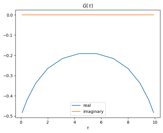
The next step in order to perform a full iteration of GF2 & GW is the evaluation of the basis representation \(G_l^F\) on the \(\tau\)-sampling points. Contrary to before when we computed \(G(\bar{\tau}_k^F)\), these sampling point will be the bosonic sampling points \(\tau_k^B\). This allows us to switch to bosonic statistic and thus be able to calculate associated quantities like the Polarization \(P\).[5]
# G_tau, bosonic
G_tau_b = tausb.evaluate(G_l_f)
pl.plot(tausb.tau,G_tau_b.real,label='real')
pl.plot(tausb.tau,G_tau_b.imag,label='imaginary')

pl.title(r'$G(\tau)$')
pl.xlabel(r'$\tau$')
pl.legend()
pl.show()
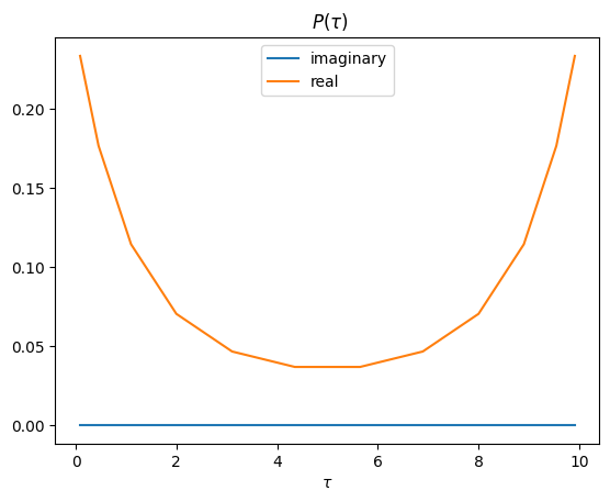
\(P(\bar\tau_k^B)\)#
The so-called Polarization \(P(\bar\tau_k^B)\) is given by the random phase approximation, a connection between two Green’s functions:
# Polarisation P, bosonic
# Note: The distribution of sampling times is symmetric around beta/2.
P_tau_b = G_tau_b * G_tau_b[::-1]
pl.plot(tausb.tau,P_tau_b.imag,label='imaginary')
pl.plot(tausb.tau,P_tau_b.real,label='real')

pl.title(r' $P(\tau)$')
pl.xlabel(r'$\tau$')
pl.legend()
pl.show()
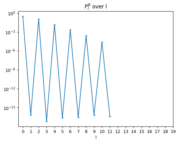
The same way we transformed \(\hat G^F(i\bar{\omega}_n^F)\) into \(G^B(\bar\tau_k^B)\) we are now able to transform \(P^B(\bar\tau_k^B)\) into \(\hat P^B(i\bar{\omega}_n^B)\) again using least Square fitting and evaluating \(P_l^B\) on the given sampling points (Matsubara frequencies).
\(P_l^B\)#
# P_l, bosonic
P_l_b = tausb.fit(P_tau_b)
pl.semilogy(np.abs(P_l_b),'+-')
pl.title('$P_l^B$ over l ')
pl.xticks(range(0,20))
pl.xlabel('l')
pl.show()
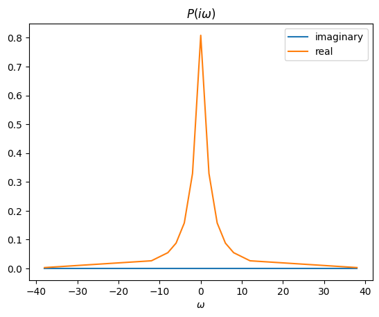
#P_iw, bosonic
P_iw_b = matsb.evaluate(P_l_b)
pl.plot(matsb.wn,P_iw_b.imag,label='imaginary')
pl.plot(matsb.wn,P_iw_b.real,label='real')
pl.title(r'$P(i\omega)$')
pl.xlabel(r'$\omega$')
pl.legend()
pl.show()
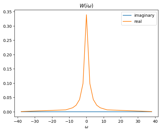
\(\hat{{W}}(i\bar{\omega}_n^B)\)#
Following \(P\) we will now calculate the Screened Interaction \(W\) with the following formula:
or
This equation has the exact same form as the Dyson equation but instead of connecting the Green’s functions and the self energy it connects the Screened Coulomb Interaction \(W\) and the polarization operator \(P\). Because \(U\) is the bare Coulomb interaction and \(P\) is an object containing all irreducible processes (meaning in Feynmann diagrams cutting an interaction line U does not result in two sides) \(W\) can be understood as the sum of all possible Feymann diagrams with an interaction U between its two parts.[5][11] This becomes quite intuitive if we look at
# W_iw, bosonic
U = 1/2

W_iw_b_U = U/(1-(U*P_iw_b))

W_iw_b = W_iw_b_U-U

#W_iw_b is the part depending on the frequency, any further calculations
#will be done using this and not W_iw_b_U
pl.plot(matsb.wn,W_iw_b.imag,label='imaginary')
pl.plot(matsb.wn,W_iw_b.real,label='real')
pl.title(r'$W(i\omega)$')
pl.xlabel(r'$\omega$')
pl.legend()
pl.show()
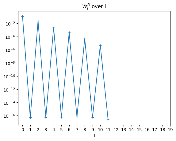
\(W_l^B\)#
# W_l, bosonic
W_l_b = matsb.fit(W_iw_b)
pl.semilogy(np.abs(W_l_b),'+-')
pl.title('$W_l^B$ over l ')
pl.xticks(range(0,20))
pl.xlabel('l')
pl.show()
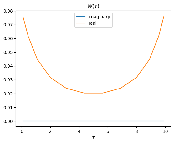
\({W}(\bar{\tau}_k^F)\)#
In the next step we are changing back into fermionic statistics:
# W_tau_f, fermionic
W_tau_f = tausf.evaluate(W_l_b)
pl.plot(tausf.tau,W_tau_f.imag,label='imaginary')
pl.plot(tausf.tau,W_tau_f.real,label='real')
pl.title(r'$W(\tau)$')
pl.xlabel(r'$\tau$')
pl.legend()
pl.show()
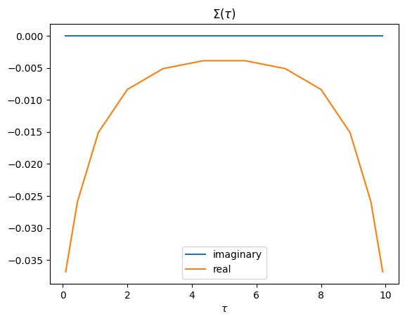
\({\Sigma}(\bar{\tau}_k^F)\)#
After changing back into fermionic statistics the next quantity that is being dealt with is the so-called self energy \(\Sigma\). When we first introduced the Dyson equation in the first chapter, we saw \(V\) as some sort of pertubation. The self-energy is very much alike as it describes the correlation effects of a many-body system. Here we will calculate \(\tilde{\Sigma}(\bar{\tau}_k^F)\) using \(\Sigma^{GW}\) so that
This can again be rewritten into its equivalent form
# E_tau , fermionic
E_tau_f = G_tau_f * W_tau_f
pl.plot(tausf.tau, E_tau_f.imag, label='imaginary')
pl.plot(tausf.tau, E_tau_f.real, label='real')
pl.title(r'$\Sigma(\tau)$')
pl.xlabel(r'$\tau$')
pl.legend()
pl.show()
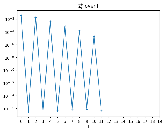
\({\Sigma}_l^F\)#
# E_l, fermionic
E_l_f = tausf.fit(E_tau_f)
pl.semilogy(np.abs(E_l_f),'+-')
pl.title('$\Sigma_l^F$ over l ')
pl.xticks(range(0,20))
pl.xlabel('l')
pl.show()
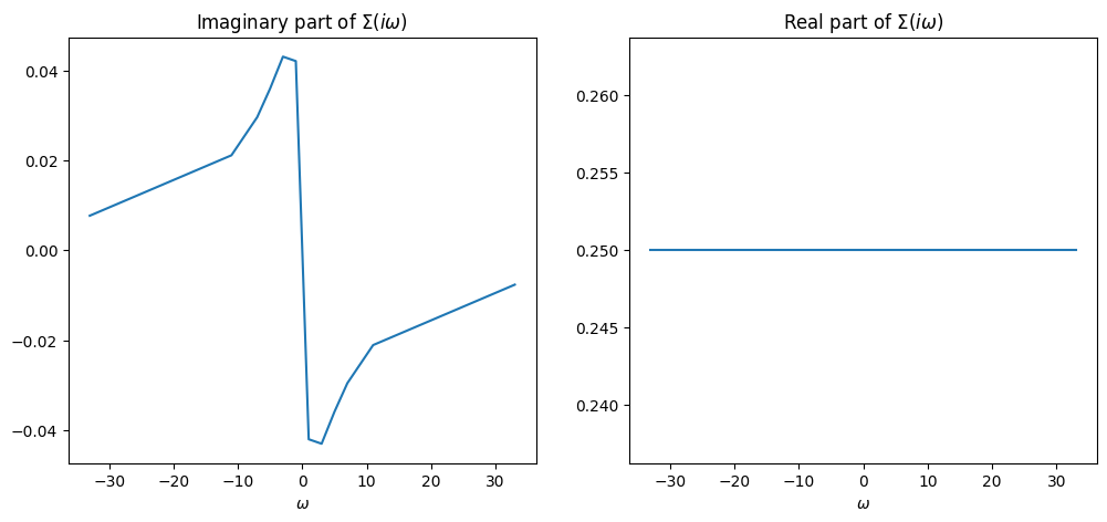
We will calculate
with \(UG(\beta)\) as the so called Hartee Fock term.
# E_iw, fermionic
E_iw_f_U = matsf.evaluate(E_l_f)-U*(basisf.u(beta).T@G_l_f)
E_iw_f = matsf.evaluate(E_l_f)


#store E_iw_f of this iteration in E_iw_f_arr
E_iw_f_arr.append(E_iw_f_U)
fig, ax = pl.subplots(1,2, figsize=(12,5) )
ax[0].plot(matsf.wn,E_iw_f_U.imag)
ax[0].set_title('Imaginary part of $\Sigma(i\omega)$')
ax[0].set_xlabel(r'$\omega$')
ax[1].plot(matsf.wn,E_iw_f_U.real)
ax[1].set_title('Real part of $\Sigma(i\omega)$')
ax[1].set_xlabel(r'$\omega$')
pl.show()
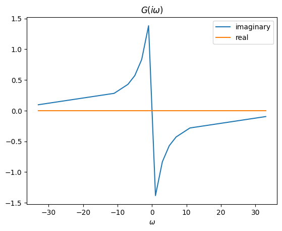
Last but not least we will obtain \(G^F(i\bar{\omega}_n^F)\) through the Dyson Equation of GW:
or
We have now calculated the full Green’s function of the system with \(\Sigma\) as a set of (one-particle) irreducible processes connected by \(G_0\).[11]
#G_iw, fermonic     -> Dyson Equation

G_iw_f = ((G_iw_0)**-1-E_iw_f)**-1
pl.plot(matsf.wn, G_iw_f.imag, label='imaginary')
pl.plot(matsf.wn, G_iw_f.real, label='real')
pl.title(r'$G(i\omega)$')
pl.xlabel(r'$\omega$')
pl.legend()
pl.show()
if (i > 0):
    pl.plot(matsf.wn, E_iw_f_arr[i].imag, label='current')
    pl.title(r'$\Sigma(i\omega)$ in the current and previous iteration')
    pl.plot(matsf.wn, E_iw_f_arr[i-1].imag, '.', label='previous')
    pl.legend()
    pl.show()
    pl.plot(matsf.wn, np.abs(E_iw_f_arr[i]-E_iw_f_arr[i-1]))
    pl.title(r'$|\Sigma_i(i\omega)-\Sigma_{i-1}(i\omega)|$' )
#Iterations
i += 1
print('full iterations: ',i)
full iterations: 1
print(G_iw_f)
[ 6.71596702e-18+0.09616324j  2.61973329e-17+0.28186928j
  1.42212771e-18+0.42789127j  9.31506612e-18+0.57065349j
 -1.35621938e-18+0.83239627j  1.22503424e-17+1.38269615j
  1.29435710e-16-1.38269615j  4.20941933e-17-0.83239627j
  2.63884962e-17-0.57065349j  1.15424968e-17-0.42789127j
  2.97349864e-17-0.28186928j  8.37563183e-18-0.09616324j]
With this we have completed one full iteration of GF2 & GW. Repeating this over and over again will show convergence and thus give the desired approximation to the self-energy.
Sources#
[1] H.Bruus, Karsten Flensberg,Many-body Quantum Theory in Condensed Matter Physics (Oxford University Press Inc., New York, 2004)
[2] J.W.Negele, H.Orland, Quantum Many-Particle Systems (Westview Press, 1998)
[3] G.D.Mahan,Many-Particle Physics (Kluwer Academic/Plenum Publishers, New York, 2000)
[4] P.C.Hansen,Dicrete Inverse Problems(Society for Industrial and Applied Mathematics, Philadelphia,2010)
[5] J.Li, M.Wallerberger, N.Chikano, C.Yeh, E.Gull and H.Shinaoka, Sparse sampling approach to efficient ab initio calculations at finite temperature, Phys. Rev. B 101, 035144 (2020)
[6] M.Wallerberger, H. Shinaoka, A.Kauch, Solving the Bethe–Salpeter equation with exponential convergence, Phys. Rev. Research 3, 033168 (2021)
[7] H. Shinaoka, N. Chikano, E. Gull, J. Li, T. Nomoto, J. Otsuki, M. Wallerberger, T. Wang, K. Yoshimi, Efficient ab initio many-body calculations based on sparse modeling of Matsubara Green’s function (2021)
[8] F. Aryasetiawan and O. Gunnarsson, The GW method, Rep. Prog. Phys. 61 (1998) 237
[9] Matteo Gatti, The GW approximation, TDDFT school, Benasque (2014)
[10]C.Friedrich, Many-Body Pertubation Theory;The GW approximation, Peter Grünberg Institut and Institute for Advanced Simulation, Jülich
[11] K. Held, C. Taranto, G. Rohringer, and A. Toschi, Hedin Equations, GW, GW+DMFT, and All That (Modeling and Simulation Vol. 1, Forschungszentrum Jülich, 2011 )