2. Tutorials¶

Sample data are provided both for fermionic and bosonic cases:

samples/fermion # a sample for fermionic spectrum (data in the SpM article)

samples/fermion_twopeak # another sample for fermionic spectrum (data in the SpM-Pade article)

samples/boson # a sample for bosonic spectrum

2.1. Fermionic system¶

Here, an explanation is given for the fermionic case (samples/fermion).

2.1.1. Script¶

User can execute all the steps explained below using a single script file run.sh. Edit some variables in the top of the script (explained later) and then run the script by

$ ./run.sh

If succeeded, text files containing numerical data and graphs in EPS format are generated in output directory. There are some parameters to control the behavior of the script;

# =========================
file_exe="../SpM.out"
dir_plt="../plt"
plot_level=1  # 0: no plot, 1: plot major data, 2: plot all data
eps_or_pdf='eps'  # 'eps' or 'pdf' (epstopdf is required)
# =========================

The fist one must be modified, at least, before running.

2.1.2. Make input files¶

Green’s function
Input data for the imaginary time Green’s function $G(\tau)$ should be provided on a linearly discretized mesh between $\tau=0$ and $\beta$ . The file Gtau.in contains sample data in the following manner
#beta=100.000000 #omega_max=4.000000 0.0 -0.500733991018 -0.499999977255 0.00025 -0.490129692246 -0.489780138726 0.0005 -0.481350067927 -0.47987901351 0.00075 -0.471476482364 -0.470285052549 0.001 -0.46176235397 -0.460987168435 ... 0.999 -0.461487347988 -0.460987168435 0.99925 -0.467256984842 -0.470285052549 0.9995 -0.479129683576 -0.47987901351 0.99975 -0.490428417896 -0.489780138726 1.0 -0.499812460744 -0.499999977255
Lines beginning with ‘#’ are skipped. There are 3 columns, which corresponds to $\tau_i/\beta$ , $G^{\rm input}(\tau_i)$ , and $G^{\rm exact}(\tau_i)$ . SpM program actually reads only one column, in this case, the second column containing $G^{\rm input}(\tau_i)$ . User is requested to specify with column parameter which column should be read. Note that the value of $G(\tau=\beta)$ needs to be given in order to evaluate the integral intensity of $\rho(\omega)$ . It means that the integrated intensity is not necessarily be equal to 1 (0 for off-diagonal Green’s function and some finite value for the self energy).
Parameters
Parameters are passed to the SpM program by a text file. The file param.in shows a setting used in obtaining the demonstrative results;
# INPUT/OUTPUT statistics="fermion" beta=100 filein_G="Gtau.in" column=1 fileout_spec="spectrum.dat" # OMEGA Nomega=1001 omegamin=-4 omegamax=4 # ADMM lambdalogbegin=2 lambdalogend=-6 tolerance=1e-10 maxiteration=1000
As in Gtau.in, lines beginning with ‘#’ are skipped. For details of each parameter and further optional parameters, see Input files

2.1.3. Run SpM¶

In the directory samples/fermion/, just type the command

$ build_directory/src/SpM.out param.in

2.1.4. Results¶

Results are stored as ordinary text format in output directory. See Output files for details of each file.

2.1.5. Plot¶

User can generate graphs either in EPS format or in PDF format using gnuplot. Move into directory output, and type

gnuplot path_to_SpM/samples/plt/*

to generate EPS files of main results. If you prefer PDF format, put flag_pdf=1 option as

gnuplot -e flag_pdf=1 path_to_SpM/samples/plt/*

Note that it requires epstopdf program in the PATH. Next, move into directory lambda_opt and type

gnuplot path_to_SpM/samples/plt/lambda_opt/*

Detailed results for the optimal value of $\lambda$ are then plotted. Again, the option flag_pdf=1 may be put to obtain PDF files.

Let us look at some graphs below.

spectrum.eps

The final result for the spectrum $\rho(\omega)$ is given in the file output/spectrum.eps.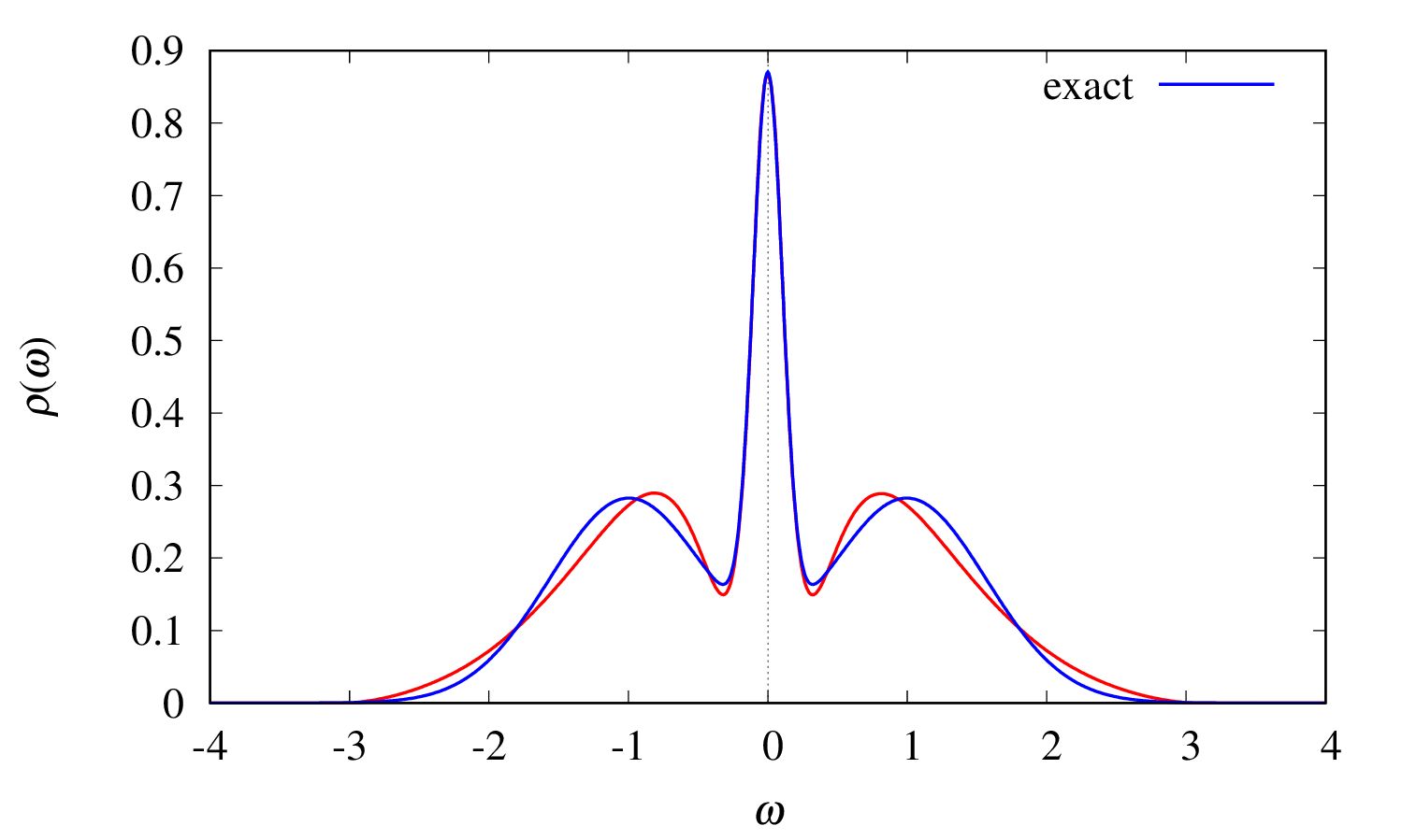

The red line shows the computed spectrum, and the blue line shows the exact spectrum, which is provided in the file Gtau.in.dos (not output of the SpM program).
find_lambda_opt.eps

User should check how the regularization parameter $\lambda$ is determined and whether the choice is reasonable. Loot at the file output/find_lambda_opt.eps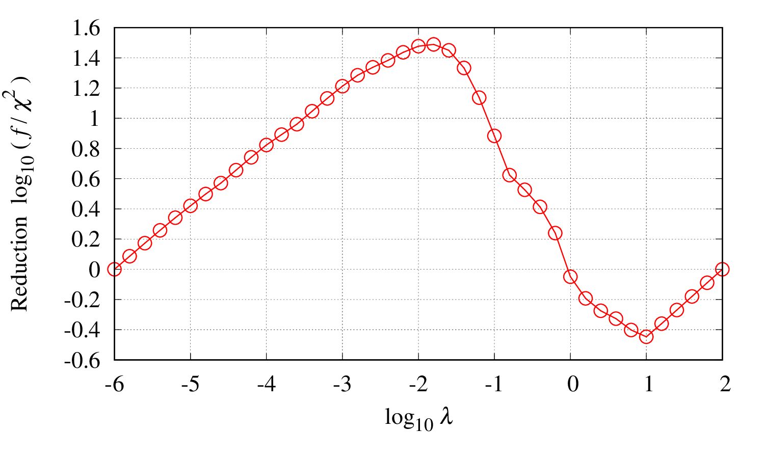

The peak position gives the optimal choice $\lambda_{\rm opt}=10^{-1.8}$ . If the peak is not clear, the choice might not be reasonable. In this case, accuracy of the input should be improved.
y_sv-log.eps

One can see how much information in the input data is used for constructing the spectrum. See the file output/lambda_opt/y_sv-log.eps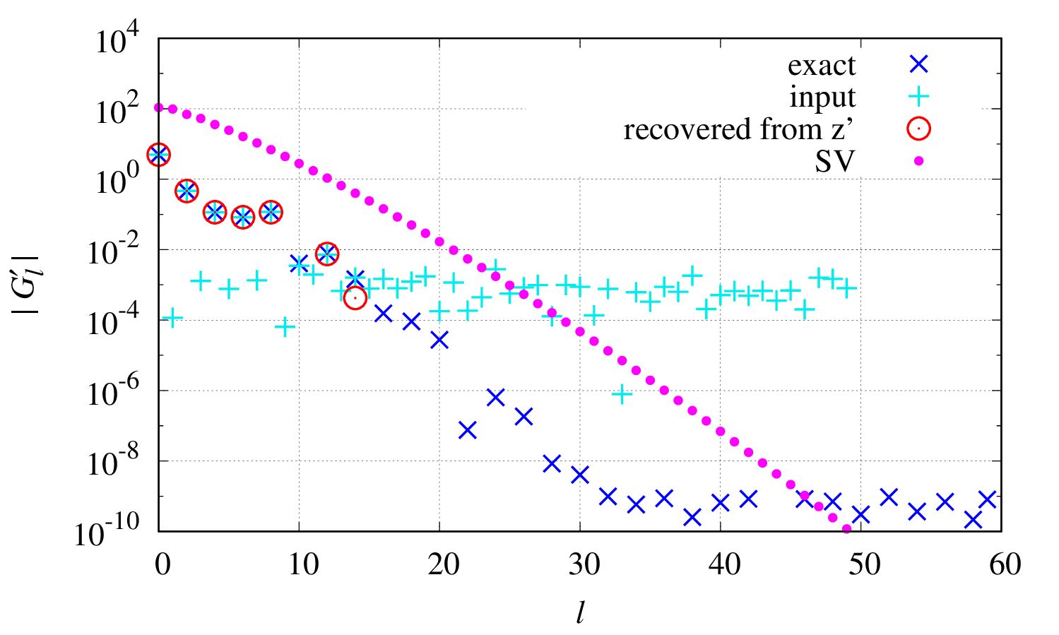

The light blue points show the input data $G'_l$ transformed into the SVD basis, and red circles are data used in computing $\rho(\omega)$ above. The blue points show, for comparison, the exact $G'_l$ without noise, which is provided in the file Gtau.in.sv_basis (not output of the SpM program).

2.2. Bosonic system¶

Sample files are available at samples/boson.

Users can deal with a bosonic system by only changing statistics parameter to "boson" from "fermion" in the parameter file.

2.3. SpM-Pade method¶

Sample files are available at samples/fermion_twopeak.

The SpM-Pade method is another SpM AC method, where unphysical oscillation in the SpM spectrum is reduced by using spectra reconstructed by the Pade AC method.

The cost function is

$L_\text{SpM-Pade}(\boldsymbol{\rho}) = L_\text{SpM}(\boldsymbol{\rho}) + \frac{\eta}{2} \sum_i w_i \left(\rho(\omega_i) - \rho^\text{Pade}(\omega_i)\right)^2,$

where

$w_i = \left(1.0 + \left(\frac{\sigma^\text{Pade}(\omega_i)}{\rho^\text{Pade}(\omega_i)}\right)^2\right)^{-1}$

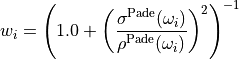
and $\rho^\text{Pade}(\omega_i)$ and $\sigma^\text{Pade}(\omega_i)$ are the expectation value and standard deviation of the spectrum reconstructed by the Pade AC method from NSamplePade Green’s functions with independent Gaussian noise. The strength of the Gaussian noise is specified by g_sigma or the pair of filein_Gsigma and column_sigma parameters (see Input files for details). The coefficient of the Pade weight, $eta$ , is specified by the PadeEta parameter. If PadeEta = 0, the original SpM method will be used.

param_spm.in and param_spmpade.in are input files for the SpM ( $\eta=0$ ) and SpM-Pade ( $\eta=1$ ) method, respectively. Note that optimal $\lambda$ for the SpM and SpM-Pade differ, and hence users may need to change the range of $lambda$ (lambdalogbegin and lambdalogend). The following figure shows the result:

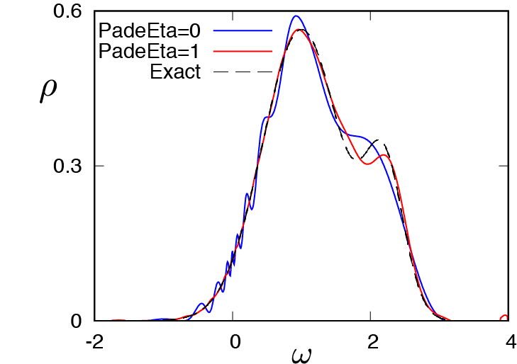
The blue curve and red curve show the spectrum reconstructed by the SpM method ( $\eta=0$ ) and the SpM-Pade method ( $\eta=1$ ), respectively. The black dashed curve shows the exact spectrum.