Sparse sampling

\[ \newcommand{\wmax}{{\omega_\mathrm{max}}} \newcommand{\dd}{{\mathrm{d}}} \newcommand{\ii}{{\mathrm{i}}} \newcommand{\iv}{{\mathrm{i}\nu}} \newcommand{\tauk}{{\bar{\tau}_k}} \newcommand{\wk}{{\bar{\omega}^\alpha_k}} \newcommand{\vk}{{\bar{\nu}_k}} \newcommand{\hatFmat}{\hat{\mathbf{F}}} \newcommand{\Fmat}{{\mathbf{F}}} \]

We consider how to compute the \(L\) expansion coefficients of a Green’s function in IR from its numerical values known on a finite set of imaginary times or imaginary frequencies. This builds on the IR expansion

\[ G(\tau) \approx \sum_{l=0}^{L-1} G_l U_l(\tau), \]

introduced in Intermediate representation (IR).

The idea of the sparse sampling is simple. If we want to determine \(L\) coefficients \(G_l\), we need to know \(G(\tau)\) on only up to \(L\) sampling points. Let \(\bar{\tau}_1 < \cdots < \bar{\tau}_{N_\mathrm{smpl}}\) (\(N_\mathrm{smpl}\ge L\)) be such sampling points, one can evaluate the expansion coefficients as

\[\begin{split} \begin{align} G_l &= \underset{G_l}{\mathrm{argmin}} \sum_k \bigg| G(\tauk) - \sum_{l=0}^{L-1} U_l(\tauk)G_l \bigg|^2\nonumber \\ &= (\Fmat^+ \boldsymbol{G})_l, \end{align} \end{split}\]

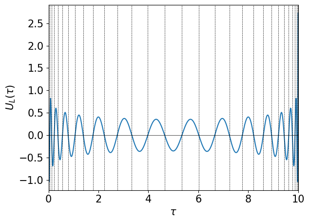
where we define \((\Fmat)_{kl} = U_l(\tauk)\) and \(\Fmat^+\) is its pseudo inverse. The numerical stability of this ``fitting’’ scheme is determined by the condition number of the coefficient matrix \(\Fmat\). An empirically good choice, which the libraries use by default, is to use the roots of \(U_L(\tau)\), the first singular function beyond the basis; they lie in \((0, \beta)\). From experience, the fitting can be done in the most stable way using SVD of the fitting matrix (already implemented in sparse-ir).

The following figure shows the default sampling points in the imaginary-time domain generated for \(\beta=10\) and \(\wmax=10\) (\(L=30\)), together with \(U_L(\tau)\), whose roots they are.

Show code cell source

Hide code cell source

import sparse_ir
import numpy as np
%matplotlib inline
import matplotlib.pyplot as plt
plt.rcParams['font.size'] = 15

beta = 10
wmax = 10
basis = sparse_ir.FiniteTempBasis("F", beta, wmax, eps=1e-10)

smpl = sparse_ir.TauSampling(basis)

# U_L, the first function beyond the basis (L = basis.size), from a larger basis for the same beta and wmax
u_L = sparse_ir.FiniteTempBasis("F", beta, wmax, eps=1e-12).u[basis.size]

taus = np.linspace(0, beta, 1000)
plt.plot(taus, u_L(taus))
plt.plot(taus, np.zeros_like(taus), ls='-', color='k', marker='', lw=0.5)
for x in smpl.sampling_points:
    plt.axvline(x=x, ls='--', lw=0.5, color='k')
plt.xlabel(r'$\tau$')
plt.ylabel(r'$U_L(\tau)$')
plt.xlim([0, beta])
plt.tight_layout()

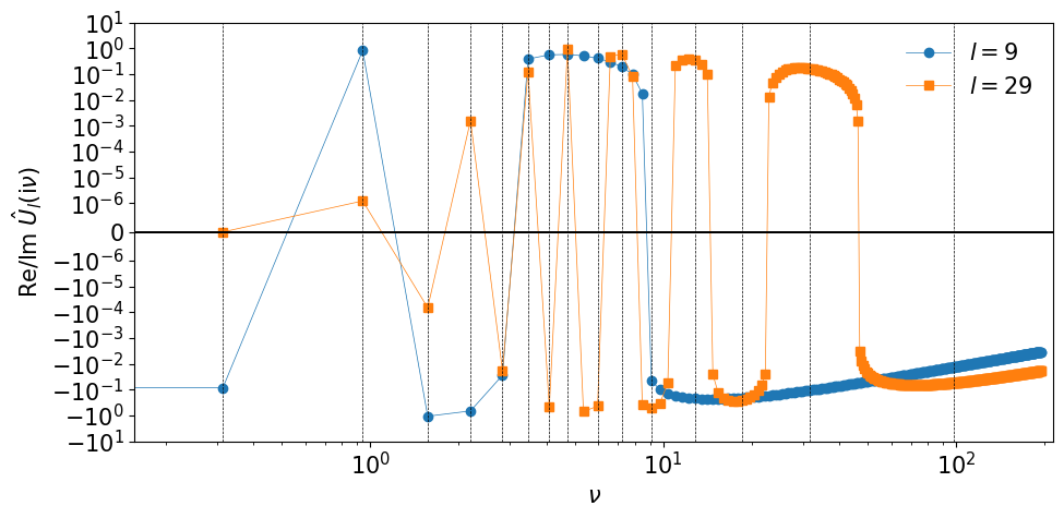
One can transform numerical data in the Matsubara-frequency domain using sparse-sampling techniques [Li et al., 2020]. For fermions, the IR basis functions \(\hat U_l(\iv)\) are purely imaginary for even \(l\) and real for odd \(l\); for bosons it is the other way round. Although the basis functions \(\hat U_l(\iv)\) are defined only on discrete points, the respective parts have sign structures similarly to those of \(U_l(\tau)\). The default sampling frequencies are the sign changes of the first discarded transform \(\hat U_l(\iv)\), with \(l \ge L\) chosen to fit the parity; bosonic sets always include \(n = 0\) (see Notation and conventions). The figure shown below shows \(\hat U_l(\iv)\) for \(l = 9\) and for the largest \(l = L-1\) of the given basis as well as the sampling frequencies. A sign change generally takes place between two adjacent Matsubara frequencies. A segment between two adjacent “roots” of \(\hat U_{L-1}(\iv)\) contains at least one sampling point.

Let \(\bar{\nu}_1 < \cdots < \bar{\nu}_{N_\mathrm{smpl}}\) (\(N_\mathrm{smpl}\ge L\)) be such sampling frequencies, one can evaluate the expansion coefficients as

\[\begin{split} \begin{align} G_l &= \underset{G_l}{\mathrm{argmin}} \sum_k \bigg| G(\ii\vk) - \sum_{l=0}^{L-1} \hat{U}_l(\ii\vk)G_l \bigg|^2\nonumber \\ &= (\hat{\Fmat}^+ \boldsymbol{G})_l. \end{align} \end{split}\]

where \((\hat{\Fmat})_{kl} = \hat U_l(\ii\vk)\). If \(G(-\iv) = G(\iv)^*\) (real coefficients \(G_l\)), MatsubaraSampling(basis, positive_only=True) samples only the non-negative frequencies \(n \ge 0\).

The following figure shows the sampling points in the imaginary-frequency domain generated for \(\beta=10\) and \(\wmax=10\).

Show code cell source

Hide code cell source

smpl_matsu = sparse_ir.MatsubaraSampling(basis)

get_nonzero_part = lambda l, data: data.imag if l%2==0 else data.real 

fig, ax = plt.subplots(figsize=(10,5))

nmax = int(2*(smpl_matsu.sampling_points.max()//2))
nvec = 2*np.arange(-nmax,nmax)+1  # reduced frequencies n (odd for fermions); nu = n*pi/beta
vvec = nvec * np.pi/beta
markers = ["o", "s"]
for idx_l, l in enumerate([9, basis.size-1]):
    ax.plot(vvec, get_nonzero_part(l, basis.uhat[l](nvec)), 
        label=f"$l={l}$", ls="-", marker=markers[idx_l], ms=6, lw=0.5)

for n in smpl_matsu.sampling_points:
    ax.axvline(n*np.pi/beta, ls="--", lw=0.5, color="k")
    ax.axhline(0, ls="-", lw=0.25, color="k")

ax.legend(frameon=False)
ax.set_xlabel(r"$\nu$")
ax.set_ylabel(r"Re/Im $\hat{U}_l(\mathrm{i}\nu)$")

ax.set_xlim([0.5*np.pi/beta, None])
ax.set_ylim([-10, 10])
ax.set_xscale("log")
ax.set_yscale("symlog", linthresh=1e-6)

plt.tight_layout()

Condition number

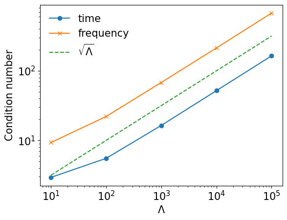
The condition number of the fitting scales roughly as \(\sqrt{\Lambda}\).

cond_tau = []
cond_matsu = []
lambdas = [1e+1, 1e+2, 1e+3, 1e+4, 1e+5]
for lambda_ in lambdas:
    basis = sparse_ir.FiniteTempBasis("F", beta, lambda_/beta, eps=1e-15)
    cond_tau.append(sparse_ir.TauSampling(basis).cond)
    cond_matsu.append(sparse_ir.MatsubaraSampling(basis).cond)

plt.loglog(lambdas, cond_tau, marker="o", label="time")
plt.loglog(lambdas, cond_matsu, marker="x", label="frequency")
plt.loglog(lambdas, np.sqrt(lambdas), marker="", ls="--", label=r"$\sqrt{\Lambda}$")
plt.xlabel(r"$\Lambda$")
plt.ylabel("Condition number")
plt.legend(frameon=False)
plt.show()