Intermediate representation (IR)

\[ \newcommand{\iv}{{\mathrm{i}\nu}} \newcommand{\wmax}{{\omega_\mathrm{max}}} \newcommand{\dd}{{\mathrm{d}}} \]

Introduction

For the definition of the Green’s function and the Lehmann representation, please refer to Green’s function and Lehmann representation.

In this document, we use the logistic kernel \(K^\mathrm{L}(\tau, \omega)\) for the singular value expansion. This kernel can be used for both fermionic and bosonic Green’s functions with appropriate modification of the spectral function (see Regularization of the bosonic kernel for details).

Our goal in this documentation is to construct a compact representation and sampling of Green’s functions on the imaginary-time axis \(\tau\) and on the Matsubara-frequency axis \(\mathrm{i}\nu\), so that a small number of basis functions and sampling points capture all relevant information.

Singular value expansion and basis functions

The singular value expnasion of the kernel (2) reads [Shinaoka et al., 2017]

\[ K^\mathrm{L}(\tau, \omega) = \sum_{l=0}^\infty U_l(\tau) S_l V_l(\omega), \]

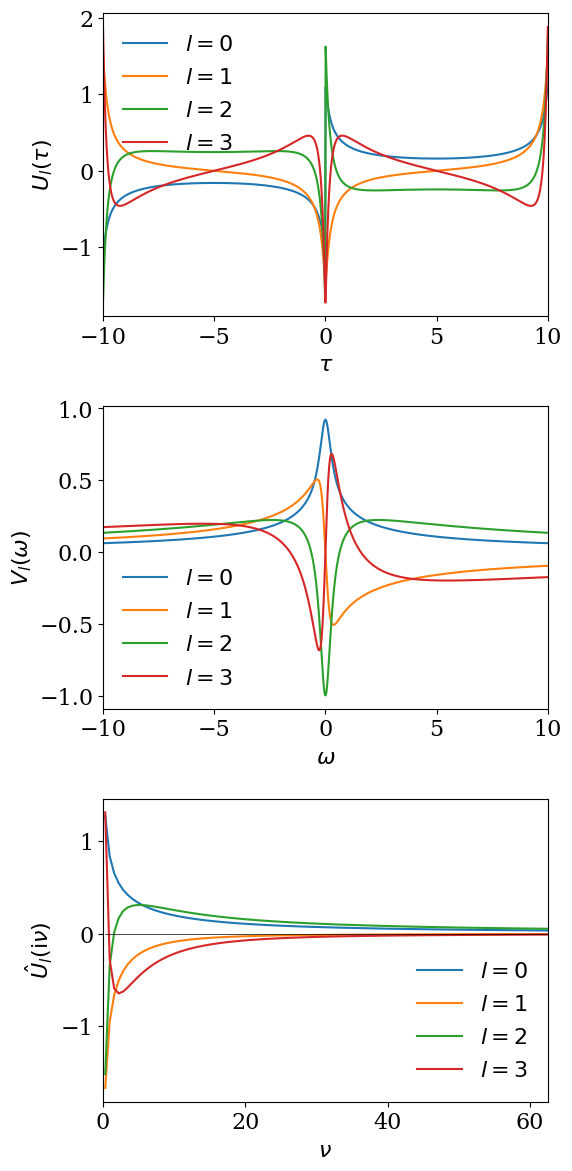
for \(\omega \in [-\wmax, \wmax]\) with \(\wmax\) (>0) being a cut-off frequency. \(U_l(\tau)\) and \(V_l(\omega)\) are left and right singular functions and \(S_l\) is the singular values (with \(S_0>S_1>S_2>...>0\)). The two sets of singular functions \(U\) and \(V\) make up the basis functions of the so-called Intermediate Representation (IR), which depends on \(\beta\) and the cutoff \(\wmax\). For the peculiar choice of the regularization for the bosonic kernel using \(K^\mathrm{L}\), these basis functions do not depend on statistical properties. The basis functions \(U_l(\tau)\) are transformed to the imaginary-frequency axis as

\[ U_l(\iv) \equiv \int_0^\beta \dd \tau e^{\iv \tau} U_l(\tau). \]

Some of the information regarding real-frequency properties of the system is often lost during transition into the imaginary-time domain, so that the imaginary-frequency Green’s function does hold less information than the real-frequency Green’s function. The reason for using IR lies within its compactness and ability to display that information in imaginary quantities.

The decay of the singular values depends on \(\beta\) and \(\wmax\) only through the dimensionless parameter \(\Lambda\equiv \beta\wmax\). In practice, we work with the non-dimensionalized kernel \(K^\mathrm{L}(x,y)\) introduced in Green’s function and Lehmann representation, where \(x = 2\tau/\beta - 1\) and \(y = \omega/\wmax\). The SVD is therefore performed once for each value of \(\Lambda\). If two problems share the same \(\Lambda = \beta\wmax\), the singular values \(S_l\) and basis functions \(U_l\), \(V_l\) can be reused. Although the SVD itself is not extremely expensive, for large cutoffs (e.g. \(\Lambda \sim 10^4\)) and high-precision settings (pseudo-multi-precision arithmetic), a single SVD can take up to \(\mathcal{O}(10)\) seconds, so reusing the result when possible is beneficial. The following plots show the singular values and the basis functions computed for \(\beta=10\) and \(\wmax=10\).

import numpy as np
%matplotlib inline
import matplotlib.pyplot as plt
import sparse_ir

plt.rcParams.update({
    "font.family": "serif",
    "font.size": 16,
})

lambda_ = 100
beta = 10
wmax = lambda_/beta
basis = sparse_ir.FiniteTempBasis('F', beta, wmax, eps=1e-10)

plt.semilogy(basis.s, marker='o', ls='')
plt.xlabel(r'$l$')
plt.ylabel(r'$S_l$')
plt.tight_layout()
plt.show()

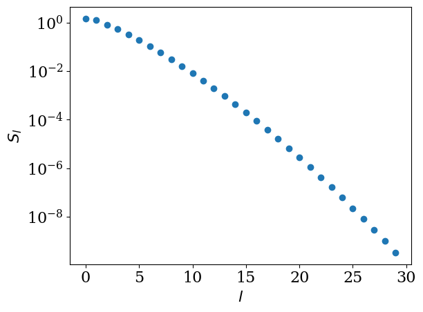
fig = plt.figure(figsize=(6,12))
ax1 = plt.subplot(311)
ax2 = plt.subplot(312)
ax3 = plt.subplot(313)
axes = [ax1, ax2, ax3]

taus = np.linspace(-beta, beta, 1000)
omegas = np.linspace(-wmax, wmax, 1000)

beta = 10
nmax = 100

v = 2*np.arange(nmax)+1
iv = 1J * (2*np.arange(nmax)+1) * np.pi/beta

uhat_val = basis.uhat(v)
for l in range(4):
    ax1.plot(taus, basis.u[l](taus), label=f'$l={l}$')
    ax2.plot(omegas, basis.v[l](omegas), label=f'$l={l}$')
    y = uhat_val[l,:].imag if l%2 == 0 else uhat_val[l,:].real
    ax3.plot(iv.imag, y, label=f'$l={l}$')

ax1.set_xlabel(r'$\tau$')
ax2.set_xlabel(r'$\omega$')
ax1.set_ylabel(r'$U_l(\tau)$')
ax2.set_ylabel(r'$V_l(\omega)$')
ax1.set_xlim([-beta, beta])
ax2.set_xlim([-wmax, wmax])

ax3.plot(iv.imag, np.zeros_like(iv.imag), ls='-', lw=0.5, color='k')
ax3.set_xlabel(r'$\nu$')
ax3.set_ylabel(r'$\hat{U}_l(\mathrm{i}\nu)$')
ax3.set_xlim([0, iv.imag.max()])

for ax in axes:
    ax.legend(loc='best', frameon=False)

plt.tight_layout()

Example: IR expansion of a simple spectral function

We expand \(G(\tau)\) and \(\rho(\omega)\) as

\[ G(\tau) = \sum_{l=0}^{L-1} G_l U_l(\tau) + \epsilon_L, \]

\[ \hat{G}(\mathrm{i}\nu) = \sum_{l=0}^{L-1} G_l \hat{U}_l(\mathrm{i}\nu) + \hat{\epsilon}_L, \]

where \(\epsilon_L,~\hat{\epsilon}_L \approx S_L\). The expansion coefficients \(G_l\) can be determined from the spectral function as

\[ G_l = -S_l \rho_l, \]

where

\[ \rho_l = \int_{-\omega_\mathrm{max}}^{\omega_\mathrm{max}} \mathrm{d} \omega \rho(\omega) V_l(\omega). \]

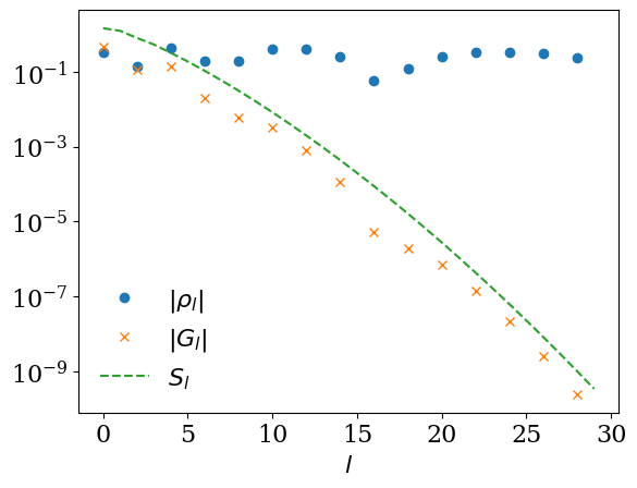
As a simple example, we consider a particle-hole-symmetric spectral function \(\rho(\omega) = \frac{1}{2} (\delta(\omega-1) + \delta(\omega+1))\) for fermions. The expansion coefficients are given by

\[ \rho_l = \frac{1}{2}(V_l(1) + V_l(-1)). \]

This example illustrates how \(|G_l|\) follows the decay of the singular values \(S_l\), so that only a small number of coefficients are numerically relevant.

rho_l = 0.5 * (np.asarray(basis.v(1)) + np.asarray(basis.v(-1)))
gl = - basis.s * rho_l

ls = np.arange(basis.size)
plt.semilogy(ls[::2], np.abs(rho_l[::2]), label=r"$|\rho_l|$", marker="o", ls="")
plt.semilogy(ls[::2], np.abs(gl[::2]), label=r"$|G_l|$", marker="x", ls="")
plt.semilogy(ls, basis.s, label=r"$S_l$", marker="", ls="--")
plt.xlabel(r"$l$")
plt.legend(frameon=False)
plt.show()
#plt.savefig("plot.pdf")

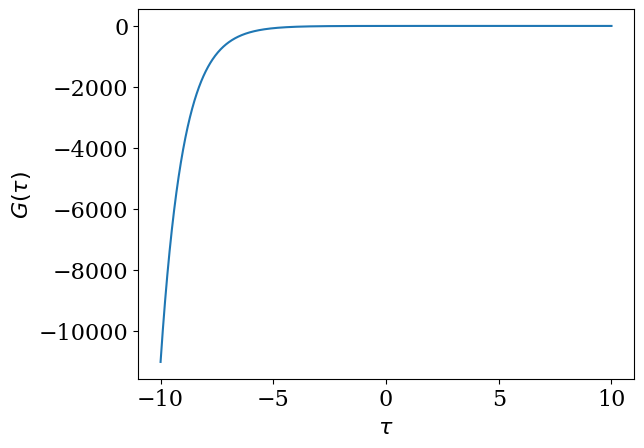
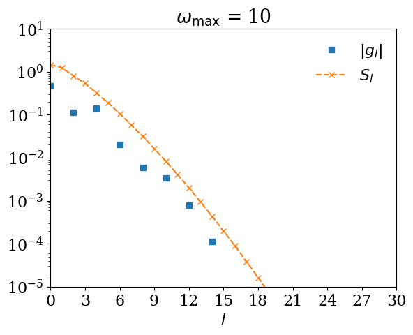
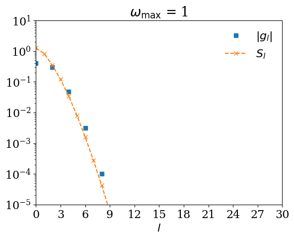
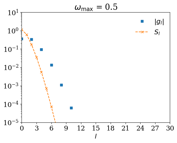
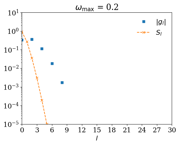
Remark: What happens if \(\omega_\mathrm{max}\) is too small?

If you expand \(G(\tau)\) using \(U_l(\tau)\) for too small \(\omega_\mathrm{max}\), \(|G_l|\) decays slower than \(S_l\). Let us demonstrate it with \(\omega_\mathrm{max} = 0.5\).

def gtau_exact(tau):
    return -0.5*(np.exp(-tau)/(1 + np.exp(-beta)) + np.exp(tau)/(1 + np.exp(beta)))

plt.plot(taus, gtau_exact(taus))
plt.xlabel(r"$\tau$")
plt.ylabel(r"$G(\tau)$")
plt.show()
#plt.savefig("gtau.pdf")

from scipy.integrate import quad
from matplotlib.ticker import MaxNLocator

for wmax_bad in [10, 1, 0.5, 0.2]:
    basis_bad = sparse_ir.FiniteTempBasis("F", beta, wmax_bad, eps=1e-10)

    # We expand G(τ).
    gl_bad = [quad(lambda x: gtau_exact(x) * basis_bad.u[l](x), 0, beta)[0] for l in range(basis_bad.size)]

    ax = plt.figure().gca()
    ax.xaxis.set_major_locator(MaxNLocator(integer=True)) # Force xtics to be integer
    plt.semilogy(np.abs(gl_bad), marker="s", ls="", label=r"$|g_l|$")
    plt.semilogy(np.abs(basis_bad.s), marker="x", ls="--", label=r"$S_l$")
    plt.title(r"$\omega_\mathrm{max}$ = " + str(wmax_bad))
    plt.xlabel(r"$l$")
    plt.xlim([0, 30])
    plt.ylim([1e-5, 10])
    plt.legend(frameon=False)
    plt.show()
    #plt.savefig(f"coeff_bad_{wmax_bad}.pdf")

Relation to Discrete Lehmann Representation (DLR)

In this page we have introduced the IR as the singular value expansion of the logistic kernel,

\[ K^\mathrm{L}(\tau, \omega) = \sum_{l=0}^\infty U_l(\tau) S_l V_l(\omega). \]

The Discrete Lehmann Representation (DLR) provides an alternative, but closely related,\n representation of Green’s functions. In the original DLR work [Kaye et al., 2022], the kernel\n is not decomposed by SVD but by an interpolative decomposition (a rank-revealing\n factorization) applied to a discretized version of \(K^\mathrm{L}(\tau, \omega)\).\n This yields a finite set of poles on the real-frequency axis and corresponding basis\n functions in \(\tau\) and Matsubara frequency.\n We do not go into the details of the interpolative decomposition here. Instead, the\n page Discrete Lehmann representation explains how the DLR can be understood\n and implemented starting from the IR basis \(U_l(\tau)\) and \(V_l(\omega)\), and how the\n resulting DLR basis is used in practice.\n

Next: sparse sampling of Green’s functions

In this chapter we have seen how Green’s functions can be represented compactly in the IR basis,

\[ G(\tau) \approx \sum_{l=0}^{L-1} G_l U_l(\tau), \qquad \hat G(\mathrm{i}\nu_n) \approx \sum_{l=0}^{L-1} G_l \hat U_l(\mathrm{i}\nu_n). \]

The next page, Sparse sampling, explains how to reconstruct the IR coefficients \(\{G_l\}_{l=0}^{L-1}\) from a small number of sampling points in imaginary time or Matsubara frequency. It shows how to choose these sampling points so that the reconstruction is numerically stable.